ENERGY_EFFICIENCY_IN_ELECTRICAL_UTILITIES
(Chapter 5:Fan & Blowers)
Introduction
Fans and blowers provide air for ventilation and industrial process requirements. Fans generate a pressure to move air (or gases) against a resistance caused by ducts, dampers, or other components in a fan system. The fan rotor receives energy from a rotating shaft and transmits it to the air.
Difference between Fans, Blowers and Compressors
Fans, blowers and compressors are differentiated by the method used to move the air, and by the system pressure they must operate against. As per American Society of |Mechanical Engineers (ASME) the specific ratio - the ratio of the discharge pressure over |the suction pressure - is used for defining the fans, blowers and compressors (see Table 5.1).

Fan Types
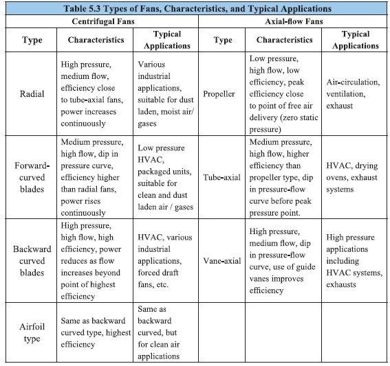
Fan and blower selection depends on the volume flow rate, pressure, type of material handled, space limitations, and efficiency. Fan efficiencies differ from design to design and also by types. Typical ranges of fan efficiencies are given in Table 5.2. Fans fall into two general categories: centrifugal flow and axial flow. In centrifugal flow, airflow changes direction twice - once when entering and second when leaving (forward curved, backward curved or inclined, radial) (see Figure 5.1). In axial flow, air enters and leaves the fan with no change in direction (propeller, tubeaxial, vaneaxial) (see Figure 5.2).

Centrifugal Fan: Types
The major types of centrifugal fan are: radial, forward curved and backward curved (see Figure 5.3).
Radial fans are industrial workhorses because of their high static pressures (upto 1400 mm WC) and
ability to handle heavily contaminated airstreams. Because of their simple design, radial fans are well
suited for high temperatures and medium blade tip speeds.
Forward-curved fans are used in clean environments and operate at lower temperatures. They are
well suited for low tip speed and high-airflow work - they are best suited for moving large volumes
of air against relatively low pressures.
Backward-inclined fans are more efficient than forward-curved fans. Backward-inclined fans reach
their peak power consumption and then power demand drops off well within their useable airflow
range. Backward-inclined fans are known as “non-overloading” because changes in static pressure do
not overload the motor.
Axial Flow Fan: Types
The major types of axial flow fans are: tube axial, vane axial and propeller (see Figure 5.4.)
Tubeaxial fans have a wheel inside a cylindrical housing, with close clearance between blade and
housing to improve airflow efficiency. The wheel turn faster than propeller fans, enabling operation
under high-pressures 250 — 400 mm WC. The efficiency is up to 65%.
Vaneaxial fans are similar to tubeaxials, but with addition of guide vanes that improve efficiency by
directing and straightening the flow. As a result, they have a higher static pressure with less dependence
on the duct static pressure. Such fans are used generally for pressures upto 500 mmWC. Vaneaxials
are typically the most energy-efficient fans available and should be used whenever possible.
Propeller fans usually run at low speeds and moderate temperatures. They experience a large change
in airflow with small changes in static pressure. They handle large volumes of air at low pressure or
free delivery. Propeller fans are often used indoors as exhaust fans. Outdoor applications include aircooled
condensers and cooling towers. Efficiency is low — approximately 50% or less.

The different types of fans, their characteristics and typical applications are given in Table 5.3.
Common Blower Types
Blowers can achieve much higher pressures than fans, as high as 1.20 kg/cm’. They are also used to
produce negative pressures for industrial vacuum systems. Major types are: centrifugal blower and
positive-displacement blower.
Centrifugal blowers look more like centrifugal pumps than fans. The impeller is typically driven and
rotates as fast as 15,000 rpm. In multi-stage blowers, air is accelerated as it passes through each impeller.
In single-stage blower, air does not take many turns, and hence it is more efficient.
Centrifugal blowers typically operate against pressures of 0.35 to 0.70 kg/cm”, but can achieve higher
pressures. One characteristic is that airflow tends to drop drastically as system pressure increases,
which can be a disadvantage in material conveying systems that depend on a steady air volume. Because of this, they are most often used in applications that are not prone to clogging.
Positive-displacement blowers have rotors, which “trap” air and push it through housing. Positivedisplacement blowers provide a constant volume of air even if the system pressure varies. They are especially suitable for applications prone to clogging, since they can produce enough pressure - typically up to 1.25 kg/cm? - to blow clogged materials free. They turn much slower than centrifugal blowers (e.g. 3,600 rpm), and are often belt driven to facilitate speed changes.
Fan Performance Evaluation and Efficient System Operation
System Characteristics
The term “system resistance” is used when referring to the static pressure. The system resistance is the
sum of static pressure losses in the system. The system resistance is a function of the configuration of ducts, pickups, elbows and the pressure drops across equipment-for example bagfilter or cyclone.The system resistance varies with the square of the volume of air flowing through the system. For a given volume of air, the fan in a system with narrow ducts and multiple short radius elbows is going to have to work harder to overcome a greater system resistance than it would in a system with larger ducts and a minimum number of long radius turns. Long narrow ducts with many bends and twists will require more energy to pull the air through them. Consequently, for a given fan speed, the fan will be able to pull less air through this system than through a short system with no elbows. Thus, the system resistance increases substantially as the volume of air flowing through the system increases; square of air flow.
Conversely, resistance decreases as flow decreases. To determine what volume the fan will produce,
it is therefore necessary to know the system resistance characteristics. In existing systems, the system resistance can be measured. In systems that have been designed, but not built, the system resistance must be calculated. Typically a system resistance curve (see Figure 5.5) is generated with for various flow rates on the x-axis and the associated resistance on the y-axis.
Fan Characteristics
Fan characteristics can be represented in form of fan curve(s). The fan curve is a performance curve
for the particular fan under a specific set of conditions. The fan curve is a graphical representation of
a number of inter-related parameters. Typically a curve will be developed for a given set of conditions
usually including: fan volume, system static pressure, fan speed, and brake horsepower required to
drive the fan under the stated conditions. Some fan curves will also include an efficiency curve so that
a system designer will know where on that curve the fan will be operating under the chosen conditions
(see Figure 5.6). In the many curves shown in the Figure, the curve static pressure (SP) vs. flow is
especially important.
The intersection of the system curve and the static pressure curve defines the operating point. When
the system resistance changes, the operating point is also changes. Once the operating point is fixed,
the power required could be found by following a vertical line that passes through the operating point
to an intersection with the power (BHP) curve. A horizontal line drawn through the intersection with
the power curve will lead to the required power on the right vertical axis. In the depicted curves, the
fan efficiency curve is also presented.
System Characteristics and Fan Curves
In any fan system, the resistance to air flow (pressure) increases when the flow of air is increased. As
mentioned before, it varies as the square of the flow. The pressure required by a system over a range
of flows can be determined and a “system performance curve” can be developed (shown as SC) (see
Figure 5.7).
This system curve can then be plotted on the fan curve to show the fan’s actual operating point at “A”
where the two curves (N1 and SC1) intersect. This operating point is at air flow Q1 delivered against
pressure P1

A fan operates along a performance given by the manufacturer for a particular fan speed. (The fan performance chart shows performance curves for a series of fan speeds.) At fan speed N , the fan will operate along the N, performance curve as shown in Figure 5.7. The fan’s actual operating point on this curve will depend on the system resistance; fan’s operating point at “A” is flow (Q1) against pressure (P1) .
Two methods can be used to reduce air flow from Q1 to Q2:
First method 1s to restrict the air flow by partially closing a damper in the system. This action causes a new system performance curve (SC,) where the required pressure is greater for any given air flow. The fan will now operate at “B” to provide the reduced air flow Q, against higher pressure P2 Second method to reduce air flow is by reducing the speed from N, to N,, keeping the damper fully pen. The fan would operate at “C” to provide the same Q, air flow, but at a lower pressure P3 Thus, reducing the fan speed is a much more efficient method to decrease airflow since less power is required and less energy is consumed.

Fan Laws
The fans operate under a predictable set of laws concerning speed, power and pressure. A change in
speed (RPM) of any fan will predictably change the pressure rise and power necessary to operate it at
the new RPM.

Fan Design and Selection Criteria
Precise determination of air-flow and required outlet pressure are most important in proper selection of fan type and size. The air-flow required depends on the process requirements; normally determined from heat transfer rates, or combustion air or flue gas quantity to be handled. System pressure requirement is usually more difficult to compute or predict. Detailed analysis should be carried out to determine pressure drop across the length, bends, contractions and expansions in the ducting system, pressure drop across filters, drop in branch lines, etc. These pressure drops should be added to any fixed pressure required by the process (in the case of ventilation fans there is no fixed pressure requirement). Frequently, a very conservative approach is adopted allocating large safety margins, resulting in over-sized fans which operate at flow rates much below their design values and, consequently, at very poor efficiency.
Once the system flow and pressure requirements are determined, the fan and impeller type are then selected. For best results, values should be obtained from the manufacturer for specific fans and impellers.
The choice of fan type for a given application depends on the magnitudes of required flow and static pressure. For a given fan type, the selection of the appropriate impeller depends additionally on rotational speed. Speed of operation varies with the application. High speed small units are generally more economical because of their higher hydraulic efficiency and relatively low cost. However, at low pressure ratios, large, low-speed units are preferable.
Fan Performance and Efficiency
Typical static pressures and power requirements for different types of fans are given in the Figure 5.8.
Fan performance characteristics and efficiency differ based on fan and impeller type (See Figure 5.9).
In the case of centrifugal fans, the hub- to-tip ratios (ratio of inner-to-outer impeller diameter) the tip
angles (angle at which forward or backward curved blades are curved at the blade tip - at the base the
blades are always oriented in the direction of flow), and the blade width determine the pressure developed by the fan.
Forward curved fans have large hub-to-tip ratios compared to backward curved fans and produce lower
pressure.
Radial fans can be made with different heel-to-tip ratios to produce different pressures.At both design and off-design points, backward-curved fans provide the most stable operation. Also, the power required by most backward —curved fans will decrease at flow higher than design values. A similar effect can be obtained by using inlet guide vanes instead of replacing the impeller with different tip angles. Radial fans are simple in construction and are preferable for high-pressure applications.Forward curved fans, however, are less efficient than backward curved fans and power rises continuously with flow. Thus, they are generally more expensive to operate despite their lower first cost. Among centrifugal fan designs, aerofoil designs provide the highest efficiency (upto 10% higher than
backward curved blades), but their use is limited to clean, dust-free air. Axial-flow fans produce lower
pressure than centrifugal fans, and exhibit a dip in pressure before reaching the peak pressure point. Axial-flow fans equipped with adjustable / variable pitch blades are also available to meet varying
flow requirements.
Propeller-type fans are capable of high-flow rates at low pressures. Tube-axial fans have medium pressure, high flow capability and are not equipped with guide vanes. Vane-axial fans are equipped with inlet or outlet guide vanes, and are characterized by high pressure,
medium flow-rate capabilities.
Performance is also dependant on the fan enclosure and duct design. Spiral housing designs with
inducers, diffusers are more efficient as compared to square housings. Density of inlet air is another
important consideration, since it affects both volume flow-rate and capacity of the fan to develop
pressure. Inlet and outlet conditions (whirl and turbulence created by grills, dampers, etc.) can
significantly alter fan performance curves from that provided by the manufacturer (which are developed
under controlled conditions). Bends and elbows in the inlet or outlet ducting can change the velocity
of air, thereby changing fan characteristics (the pressure drop in these elements is attributed to the
system resistance). All these factors, termed as System Effect Factors, should, therefore, be carefully
evaluated during fan selection since they would modify the fan performance curve.
Centrifugal fans are suitable for low to moderate flow at high pressures, while axial-flow fans are
suitable for low to high flows at low pressures. Centrifugal fans are generally more expensive than
axial fans. Fan prices vary widely based on the impeller type and the mounting (direct-or-belt-coupled,
wall-or-duct-mounted). Among centrifugal fans, aerofoil and backward-curved blade designs tend to
be somewhat more expensive than forward-curved blade designs and will typically provide more
favourable economics on a lifecycle basis. Reliable cost comparisons are difficult since costs vary
with a number of application-specific factors. A careful technical and economic evaluation of available
options is important in identifying the fan that will minimize lifecycle costs in any specific application.
Safety margin
The choice of safety margin also affects the efficient operation of the fan. In all cases where the fan
requirement is linked to the process/other equipment, the safety margin is to be decided, based on the
discussions with the process equipment supplier. In general, the safety margin can be 5 % over the
maximum requirement on flow rate.
In the case of boilers, the induced draft (ID) fan can be designed with a safety margin of 20 % on volume and 30 % on head. The forced draft (FD) fans and primary air (PA) fans do not require any safety margins. However, safety margins of 10 % on volume and 20 % on pressure are maintained for FD and PA fans.
System Resistance and Pressure Drop
The system resistance has a major role in determining the performance and efficiency of a fan. The system resistance also changes depending on the process. For example, the formation of the coatings / erosion of the lining in the ducts, changes the system resistance marginally. In some cases, the change of equipment (e.g. Replacement of Multi-cyclones with ESP / Installation of low pressure drop cyclones in cement industry) duct modifications, drastically shift the operating point, resulting in lower fficiency.
In such cases, to maintain the efficiency as before, the fan has to be changed. Hence, the system resistance has to be periodically checked, more so when modifications are introduced and action taken accordingly, for efficient operation of the fan.
System resistance in the application of centrifugal fan is the resistance offered by all the process equipment and duct line connected to the inlet of the fan as well as at the out let of the fan, usually stacks. In the Figure 5.10 draft required to overcome the resistance offered by the boiler to draw the flue gases -10 mmWe (- ve sign indicates the suction), the draft required to draw the flue gases through the economiser, Air heater and dust control system are added to estimate the total resistance at the inlet of the ID fan (i.e. -10 — 30 -40 — 150 =- 230 mmWc). However the ID fan requires a minimum of 10 mmWe pressure to push the gases to the bottom of the stack from where the gases will be taken care by natural draft into atmosphere. Hence the overall resistance (pressure drop) to be build up by the ID fan is the difference between the outlet pressure and the inlet pressure [i.e. 10 — (-230) = 240 mmWc].

System resistance is a function of gas density and the velocity of the gas. In the Figure 5.10 initially when there is no flue gas generation, there is no gas velocity in the process equipment and the ducts and hence the resistance (pressure drop) is zero (see Figure 5.11). After the boiler firing is started, there is continuous increase in the generation of flue gases and accordingly there is continuous increase in the velocity of the gases and continuous increase in draft. When the boiler is fired at rated capacity, the generation of flue gases are maximum resulting in corresponding pressure drop, which is the “operating point” ( 30,000 m*/hr, 240 mmWc) of the boiler ( Figure 5.11). Accordingly the ID fan with a characteristic (Performance) curve passing through the “operating point” of the system at the highest possible fan efficiency has to be selected for better utilisation of energy.

Flow Control Strategies
Typically, once a fan system is designed and installed, the fan operates at a constant speed. There may
be occasions when a speed change 1s desirable, i.e., when adding a new run of duct that requires an
increase in air flow (volume) through the fan. There are also instances when the fan is oversized and
flow reductions are required.
Various ways to achieve change in flow are: pulley change, damper control, inlet guide vane control,
variable speed drive and series and parallel operation of fans.
Pulley Change
When a fan volume change is required on a permanent basis, and the existing fan can handle the change
in capacity, the volume change can be achieved with a speed change. The simplest way to change the speed is with a pulley change. For this, the fan must be driven by a motor through a v-belt system. The fan speed can be increased or decreased with a change in the drive pulley or the driven pulley or in some cases,both pulleys. As shown in the Figure 5.12, a higher sized fan operating with damper control was downsized by reducing the motor (drive) pulley size from 8” to 6”. The power reduction was 12 kW.

Damper Controls
Some fans are designed with damper controls (see Figure 5.13). Dampers can be located at inlet or outlet. Dampers provide a means of changing air volume by adding or removing system resistance. This resistance forces the fan to move up or down along its characteristic curve, generating more or less air
without changing fan speed. However, dampers provide a limited amount of adjustment, and they are not particularly energy efficient.
Inlet Guide Vanes
Inlet guide vanes are another mechanism that can be used to meet variable air demand (see Figure .14). Guide vanes are curved sections that lay against the inlet of the fan when they are open. When they are closed, they extend out into the air stream. As they are closed, guide vanes pre-swirl the air entering the fan housing. This changes the angle at which the air is presented to the fan blades, which, in turn, changes the characteristics of the fan curve. Guide vanes are energy efficient for modest flow reductions — from 100 percent flow to about 80 percent. Below 80 percent flow, energy efficiency drops sharply.
Axial-flow fans can be equipped with variable pitch blades, which can be hydraulically or pneumatically controlled to change blade pitch, while the fan is at stationary. Variablepitch blades modify the fan characteristics substantially and thereby provide dramatically higher energy efficiency than the other options discussed thus far.
Variable Speed Drives
Although, variable speed drives are expensive, they provide almost infinite variability in speed control.
Variable speed operation involves reducing the speed of the fan to meet reduced flow requirements.
Fan performance can be predicted at different speeds using the fan laws. Since power input to the fan
changes as the cube of the flow, this will usually be the most efficient form of capacity control. However, variable speed control may not be economical for systems, which have infrequent flow variations. When considering variable speed drive, the efficiency of the control system (fluid coupling, eddycurrent, VFD, etc.) should be accounted for, in the analysis of power consumption.
Series and Parallel OperationParallel operation of fans is another useful form of capacity control. Fans in parallel can be additionally
equipped with dampers, variable inlet vanes, variable pitch blades, or speed controls to provide a high degree of flexibility and reliability.
Combining fans in series or parallel can achieve the desired airflow without greatly increasing the system package size or fan diameter. Parallel operation is defined as having two or more fans blowing together side by side.
The performance of two fans in parallel will result in doubling the volume flow, but only at free delivery. As Figure 5.15 shows, when a system curve is overlaid on the parallel performance curves, the higher the system resistance, the less increase in flow results with parallel fan operation. Thus, this type of application should only be used when the fans can operate in a low resistance almost in a free delivery condition.
Series operation can be defined as using multiple fans in a push-pull arrangement. By staging two fans
in series, the static pressure capability at a given airflow can be increased, but again, not to double at
every flow point, as the above Figure displays. In series operation, the best results are achieved in
systems with high resistances.
In both series and parallel operation, particularly with multiple fans certain areas of the combined
performance curve will be unstable and should be avoided. This instability is unpredictable and is a
function of the fan and motor construction and the operating point.
Factors to be considered in the selection of flow control methods
Comparison on of various volume control methods with respect to power consumption (%) required power is shown in Figure 5.16.
All methods of capacity control mentioned above have turn-down ratios (ratio of maximum-—to— minimum flow rate) determined by the amount of leakage (slip) through the control elements. For example, even with dampers fully closed, the flow may not be zero due to leakage through the damper. In the case of variable-speed drives the turn-down ratio is limited by the control system. In many cases, the minimum possible flow will be determined by the characteristics of the fan itself. Stable operation of a fan requires that it operate in a region where the system curve has a positive slope and the fan curve has a negative slope.
The range of operation and the time duration at each operating point also serves as a guide to selection of the most suitable capacity control system. Outlet damper control due to its simplicity, ease of operation, and low investment cost, is the most prevalent form of capacity control. However, it is the most inefficient of all methods and is best suited for situations where only small, infrequent changes are required (for example, minor process variations due to seasonal changes. The economic advantage of one method over the other is determined by the time duration over which the fan operates at different operating points. The frequency of flow change is another important determinant. For systems requiring frequent flow control, damper adjustment may not be convenient. Indeed, in many plants, dampers are not easily accessible and are left at some intermediate position to avoid frequent control.
Fan Performance Assessment
The fans are tested for field performance by measurement of flow, head and temperature on the fan side and electrical motor kW input on the motor side.
Air flow measurement
Static pressure
Static pressure is the potential energy put into the system by the fan. It is given up to friction in the ducts and at the duct inlet as it is converted to velocity pressure. At the inlet to the duct, the static pressure produces an area of low pressure (see Figure 5.17).
Velocity pressure
Velocity pressure is the pressure along the line of the flow that results from the air flowing through the
duct. The velocity pressure is used to calculate air velocity.
Total pressure
Total pressure is the sum of the static and velocity pressure. Velocity pressure and static pressure can change as the air flows though different size ducts accelerating and de-accelerating the velocity. The total pressure stays constant, changing only with friction losses. The illustration that follows shows how the total pressure changes in a system.
The fan flow is measured using pitot tube manometer combination, or a flow sensor (differential pressure instrument) or an accurate anemometer. Care needs to be taken regarding number of traverse points, straight length section (to avoid turbulent flow regimes of measurement) up stream and downstream of measurement location. The measurements can be on the suction or discharge side of the fan and preferably both where feasible.
Measurement by Pitot tube
The Figure 5.18 shows how velocity pressure is measured using a pitot tube and a manometer. Total pressure is measured using the inner tube of pitot tube and static pressure is measured using the outer tube of pitot tube. When the inner and outer tube ends are connected to a manometer, we get the velocity pressure. For measuring low velocities, it is preferable to use an inclined tube manometer instead of U tube manometer.
Measurements and Calculations
Velocity pressure/velocity calculation
When measuring velocity pressure the duct diameter (or the circumference from which to calculate the diameter) should be measured as well. This will allow us_ to calculate the velocity and the volume of air in the duct. In most cases, velocity must be measured at several places in the same system. The velocity pressure varies across the duct. Friction slows the air near the duct walls, so the velocity is greater in the center of the duct. The velocity is affected by changes in the ducting configuration such as bends and curves. The best place to take measurements is in a section of duct that is straight for at least 3-5 diameters after any elbows, branch entries or duct size changes

To determine the average velocity, it is necessary to take a number of velocity pressure readings across the cross-section of the duct. The velocity should be calculated for each velocity pressure reading, and the average of the velocities should be used. Do not average the velocity pressure; average the velocities. For round ducts over 6 inches diameter, the following locations will give areas of equal concentric area (see Figure 5.19).
For best results, one set of readings should be taken in one direction and another set at a 90° angle to the first. For square ducts, the readings can be taken in 16 equally spaced areas. If it is impossible to traverse the duct, an approximate average velocity can be calculated by measuring the velocity pressure in the center of the duct and calculating the velocity. This value is reduced to an approximate average by multiplying by 0 .9.
Calculation of Velocity: After taking velocity pressures readings, at various traverse points, the velocity corresponding to each point is calculated using the following expression.
EXAMPLE
Air flow measurements using the pitot tube, in the primary air fan of a coal fired boiler gave the
following data, calculate the velocity of air.
Air temperature = 38°C
Velocity pressure = 47mmWC
Pitot tube constant,Cp = 0.9
Air density at 38°C = 1.135 kg/m
Find out the velocity of air in m/sec
Calculation of gas density
To calculate the velocity and volume from the velocity pressure measurements, it is necessary to know
the density of gas. The density is dependent on altitude, temperature, molecular weight and pressure.
Calculation of molecular weight for flue gas consisting of CO2, CO, O2, N2 (M) (dry basis), kg/
kg mole
Volume calculation
The volume in a duct can be calculated for the velocity using the equation:
Fan efficiency
Fan manufacturers generally use two ways to mention fan efficiency: mechanical efficiency (sometimes
called the total efficiency) and static efficiency. Both measure how well the fan converts horsepower into flow and pressure The equation for determining mechanical efficiency is:
The static efficiency equation is the same except that the outlet velocity pressure is not added to the
fan static pressure

Drive motor kW can be measured by a load analyzer. This kW multiplied by motor efficiency gives the shaft power to the fan.
Energy Savings Opportunities
Minimizing demands on the fan.
1. Minimising excess air level in combustion systems to reduce FD fan and ID fan load.
2. Minimising air in-leaks in hot flue gas path to reduce ID fan load, especially in case of kilns, boiler plants, furnaces, etc. Cold air in-leaks increase ID fan load tremendously, due to density increase of flue gases and in-fact choke up the capacity of fan, resulting as a bottleneck for boiler / furnace itself.
3. In-leaks/out-leaks in air conditioning systems also have a major impact on energy efficiency and fan power consumption and need to be minimized.
The findings of performance assessment trials will automatically indicate potential areas for improvement, which could be one or a more of the following:
1. Change of impeller by a high efficiency impeller along with cone.
2.Change of fan assembly as a whole, by a higher efficiency fan
3.Impeller derating (by a smaller dia impeller)
4.Change of metallic / Glass reinforced Plastic (GRP) impeller by the more energy efficient hollow FRP impeller with aerofoil design, in case of axial flow fans, where significant savings have been reported
5. Fan speed reduction by pulley dia modifications for derating
6. Option of two speed motors or variable speed drives for variable duty conditions
7. Option of energy efficient flat belts, or, cogged raw edged V belts, in place of conventional
V belt systems, for reducing transmission losses.
8. Adopting inlet guide vanes in place of discharge damper control
9. Minimizing system resistance and pressure drops by improvements in duct system
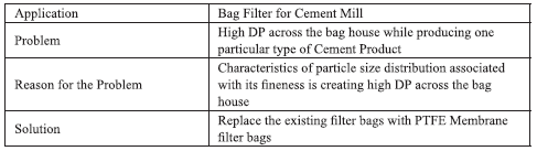
Case Study on Pressure Drop Reduction Across the Bag Filter
One of the Cement filter bag house is experiencing high Differential Pressure (DP) across the bag house while producing one particular type of cement. This high DP is resulting in high power consumption and puffing from the bag house. Upon examination it has been found that particle size distribution for this particular type of Cement associated with the fineness is creating high DP. The results of this replacement are self explanatory in the details given below:
Case Studies VSD Applications
Case 1: Cement plants use a large number of high capacity fans. By using liners on the impellers,
which can be replaced when they are eroded by the abrasive particles in the dust-laden air, the plants
have been able to switch from radial blades to forward-curved and backward-curved centrifugal fans.
This has vastly improved system efficiency without requiring frequent impeller changes. For example, a careful study of the clinker cooler fans at a cement plant showed that the flow was much higher than required and also the old straight blade impeller resulted in low system efficiency.
It was decided to replace the impeller with a backward-curved blade and use liners to prevent erosion
of the blade. This simple measure resulted in a 53 % reduction in power consumption, which amounted
to annual savings of Rs. 2.1 million.
Case 2: Another cement plant found that a large primary air fan which was belt driven through anrrangement of bearings was operating at system efficiency of 23 %. The fan was replaced with a direct coupled fan with a more efficient impeller. Power consumption reduced from 57 kW to 22 kW. Since cement plants use a large number of fans, it is generally possible to integrate the system such that air can be supplied from a common duct in many cases.
For example, a study indicated that one of the fans was operated with the damper open to only 5 %.
By re-ducting to allow air to be supplied from another duct where flow was being throttled, it was
possible to totally eliminate the use of a 55 kW fan.
Case 3: The use of variable-speed drives for capacity control can result in significant power savings.
A 25 ton-per-hour capacity boiler was equipped with both an induced-draft and forced-draft fan. Outlet
dampers were used to control the airflow. After a study of the air-flow pattern, it was decided to install
a variable speed drive to control air flow. The average power consumption was reduced by nearly 41
kW resulting in annual savings of Rs. 0.33 million. The investment of Rs. 0.65 million for the variablespeed drive was paid back in under 2 years.
Case 4: The type of variable-speed drive employed also significantly impacts power consumption.
Thermal power stations install a hydraulic coupling to control the capacity of the induced-draft fan.
It was decided to install a VFD on ID fans in a 200 MW thermal power plant. A comparison of the
power consumption of the two fan systems indicated that for similar operating conditions of flow and
plant power generation, the unit equipped with the VFD control unit consumed, on average, 4 million
units / annum less than the unit equipped with the hydraulic coupling.
Computational Fluid Dynamics
Use of Computational Fluid Dynamics (CFD) for Energy Efficiency
Computational Fluid Dynamics (CFD) is a powerful computer based simulation tool, which uses mathematics to model the physical system and to solve equations to predict the mass, momentum and energy. CFD tools helps to visualize the flow pattern, temperature and pressure profiles as well as particle movement inside the equipment / system under consideration. Being a simulation tool, various designs / operating parameters can be changed to arrive at best operating conditions for the plant. This also helps to determine the effect of changes in key process parameters before making any changes in the manufacturing process at plant.
Since it is a proactive analysis and design tool, it can highlight the root cause not just the effect when
evaluating plant problems. It is able to reduce scale-up problems because the models are based on fundamental physics and are scale independent. It is also useful in simulating conditions where it is not possible to take detailed measurements because of high temperature or dangerous environment.
Application of CFD in a Fan System for Energy Efficiency
In addition to optimization of the fan itself, the upstream and downstream flow situations are important
for trouble free operation of the fan and maximum possible efficiency. If, for instance, the incoming
flow is turbulent or swirling because of poorly designed bends or changes in cross-section, this will
affect the fan’s operating characteristics. Disturbances in the inflow and outflow zones have particularly
serious effects in the case of high efficiency fans (> 80 %); as such fans depend on a non-swirling
inflow in order to achieve their efficiency figures.
This case study describes the optimization of the induced draught flow of a double-inlet fan using
CFD. Figure 5.20 shows the system arrangement drawing. The 3D model derived from this drawing
is Shown in Figure 5.21. The very sharp-edged transitions at inlet side affect the smooth flow.
The simulation (Figure 5.22) shows extensive flow disruption and instability. The pressure drop of
this system is correspondingly high. From the inlet until the end of the first branch, the pressure drop
is about 260 Pa. From the inlet until the next branch the drop is as high as 430 Pa because of the flow
disruption near the end of the horizontal duct.
The black circles indicate unfavourable situations because this design involves transitions that are too
sharp-edged and thus prevent the flow from following the contours, resulting in turbulence. This causes
pressure drops and thus leads to additional electrical energy consumption. By contrast, the white circle
indicates a duct end producing an inefficient fluid flow.
Since a portion of the vortex flow is sucked into the fan it has to cope with strongly swirling inflow
air and therefore loses efficiency and suffers from mechanical vibrations.
Optimization of the geometry involved redesigning the critical points highlighted in Figure 5.22 so that the cross-section transitions were smooth. This redesigning succeeded in reducing the pressure drop at the front inflow duct to the fan by a factor of four, from 261 Pa to 66 Pa, while the pressure drop at the rear inflow duct that had been caused by the poorly-designed horizontal duct end (Figure 5.22, white circle) was even reduced to little more than one sixth the original figure. The severe swirling of the fan intake air (Figure 5.23, red circles) was also significantly reduced, enabling the fan to achieve its rated performance figures. The mean pressure drop saving of 275 Pa at a volume flow of 5,00,000 m3/h significantly reduces the power consumption. The resultant power saving was of the order of 49 kW.
Solved Example:
A V-belt centrifugal fan is supplying air to a process plant. The performance test on the fan gave the
following parameters.
Find out the static fan efficiency.
Ans:
------------------------------


Comments
Post a Comment