ENERGY_EFFICIENCY_IN_ELECTRICAL_UTILITIES
(Chapter 1: Electrical System)
Introduction to Electric Power Supply Systems
Electric power supply system comprises of generating units that produce electricity; high voltage
transmission lines that transport electricity over long distances; distribution lines that deliver the
electricity to consumers; substations that connect the pieces to each other; and energy control centers
to coordinate the operation of the components.
The Figure 1.1 shows a simple electric supply system with Generating Station, Power transmission
and distribution network and linkages from electricity sources to end-user.

Power Generation Plant
The fossil fuels such as coal, oil and natural gas, nuclear energy, and falling water (hydel) are commonly
used energy sources in the power generating plant. A wide and growing variety of unconventional
generation technologies and fuels have also been developed, including cogeneration, solar energy,
wind generators, and waste materials. About 70 % of power generating capacity in India is from coal based thermal power plants. The
principle of coal-fired power generation plant is shown in Figure 1.2. Energy stored in the coal
is converted in to electricity in a thermal power plant. Coal is pulverized to the consistency of talcum
powder. Then powdered coal is blown into the water wall boiler where it is burned at temperature
higher than 1300°C. The heat in the combustion gas is transferred into steam. This high-pressure steam
is used to spin the steam turbine. Finally turbine rotates the generator to produce electricity.

In India, for the coal based power plants, the overall efficiency ranges from 28% to 35% depending
upon the size, operational practices, fuel quality and capacity utilization. Where fuels are the source
of generation, a common term used is the “HEAT RATE” which reflects the efficiency of generation.
“HEAT RATE” is the heat input in kilo Calories or kilo Joules, for generating ‘one’ kilo Watt-hour of
electrical output. One kilo Watt hour of electrical energy being equivalent to 860 kilo Calories of
thermal energy or 3600 kilo Joules of thermal energy. The “HEAT RATE” is inversely proportional
to efficiency of power generation 1.e., lower the heat rate, higher is the generation efficiency.
Transmission and Distribution Lines:
The power plants typically produce 50 cycle/second (Hertz),
alternating-current (AC) electricity with voltages between 11kV
and 33kV. At the power plant site, the 3-phase voltage is stepped ;
up to a higher voltage for transmission on cables strung on cross- 2 sae
country towers.
High voltage (HV) and extra high voltage (EHV) transmission is
the next stage from power plant to transport A.C. power over long
distances at voltages like; 220 kV & 400 kV (Figure 1.3). Where
transmission is over 1000 kM, high voltage direct current
transmission is also favored to minimize the losses.

Sub-transmission network at 132 kV, 110 kV, 66 kV or 33 kV
constitutes the next link towards the end user. Distribution at 11 kV/6.6kV/3.3 kV constitutes the last link to the consumer, who is connected directly or through transformers
depending upon the drawn level of service. The transmission and distribution network include sub-stations,
lines and distribution transformers. High voltage transmission is used so that smaller, more economical wire
sizes can be employed to carry the lower current and to reduce losses. Sub-stations, containing step-down
transformers, reduce the voltage for distribution to industrial users. The voltage is further reduced for
commercial facilities. Electricity must be generated, as and when it is needed since electricity cannot be
stored virtually in the system. Typical voltage levels in a power system are given in Figure 1.4.

There is no difference between a transmission line and a distribution line except for the voltage level
and power handling capability. Transmission lines are usually capable of transmitting large quantities
of electric energy over great distances. They operate at high voltages. Distribution lines carry limited
quantities of power over shorter distances.
Voltage drops in line are in relation to the resistance and reactance of line, length and the current drawn.
For the same quantity of power handled, lower the voltage, higher the current drawn and higher the voltage
drop. The current drawn is inversely proportional to the voltage level for the same quantity of power handled.
The power loss in line is proportional to resistance and square of current. (i.e. P, , =I’R). Higher voltage
transmission and distribution thus would help to minimize line voltage drop in the ratio of voltages,
and the line power loss in the ratio of square of voltages. For instance, if distribution of power is raised
from 11 kV to 33 kV, the voltage drop would be lower by a factor 1/3 and the line loss would be lower
by a factor (1/3) i.e., 1/9. Lower voltage transmission and distribution also calls for bigger size
conductor on account of current handling capacity needed.
Cascade Efficiency
The primary function of transmission and distribution equipment is to transfer power economically
and reliably from one location to another.
Conductors in the form of wires and cables strung on towers and poles carry the high-voltage, AC
electric current. A large number of copper or aluminum conductors are used to form the transmission
path. The resistance of the long-distance transmission conductors is to be minimized. Energy loss in
transmission lines is wasted in the form of I’R losses.
Capacitors are used to correct power factor by causing the current to lead the voltage. When the AC currents
are kept in phase with the voltage, operating efficiency of the system is maintained at a high level.
Circuit-interrupting devices are switches, relays, circuit breakers, and fuses. Each of these devices is
designed to carry and interrupt certain levels of current. Making and breaking the current carrying
conductors in the transmission path with a minimum of arcing is one of the most important characteristics
of this device. Relays sense abnormal voltages, currents, and frequency and operate to protect the system.
Transformers are placed at strategic locations throughout the system to minimize power losses in the
T&D system. They are used to change the voltage level from low-to-high in step-up transformers and
from high-to-low in step-down units.
The power source to end user energy efficiency link is a key factor, which influences the energy input at the
source of supply. If we consider the electricity flow from generation to the user in terms of cascade energy
efficiency, typical cascade efficiency profile from generation to 11 — 33 kV user industry will be as follows:

The cascade efficiency in the T&D system from output of the power plant to the end use is 87% (i.e.
0.995 x 0.99 x 0.975 x 0.96 x 0.995 x 0.95 = 87%)
After power generation at the plant it is transmitted and distributed over a wide network. The standard
technical losses are around 17 % in India (Efficiency=83%). But the figures for many of the states
show T & D losses ranging from 17 — 50 %. All these may not constitute technical losses, since unmetered and pilferage are also accounted in this loss.
Industrial End User
At the industrial end user premises, again the plant network elements like transformers at receiving
sub-station, switchgear, lines and cables, load-break switches, capacitors cause losses, which affect
the input-received energy. However the losses in such systems are meager and unavoidable.
A typical plant single line diagram of electrical distribution system is shown in Figure 1.5

When the power reaches the industry, it meets the transformer. The energy efficiency of the transformer
is generally very high. Next, it goes to the motor through internal plant distribution network. A typical
distribution network efficiency including transformer is 95% and motor efficiency is about 90%.
Another 30 % (Efficiency=70%) is lost in the mechanical system which includes coupling/ drive train,
a driven equipment such as pump and flow control valves/throttling etc. Thus the overall energy
efficiency becomes 50%. (0.83 x 0.95x 0.9 x 0.70 = 0.50, i.e. 50% efficiency)
Hence one unit saved in the end user is equivalent to two units generated in the power plant.
(1Unit / 0.5Eff = 2 Units)
Electricity Billing
The electricity billing by utilities for medium & large enterprises, in High Tension (HT) category, is
often done on two-part tariff structure, i.e. one part for capacity (or demand) drawn and the second
part for actual energy drawn during the billing cycle. Capacity or demand is in kVA (apparent power)
or kW terms. The reactive energy (i.e.) kVArh drawn by the service is also recorded and billed for in
some utilities, because this would affect the load on the utility. Accordingly, utility charges for maximum
demand, active energy and reactive power drawn (as reflected by the power factor) in its billing
structure. In addition, other fixed and variable expenses are also levied.
The tariff structure generally includes the following components:
a) Maximum demand Charges
These charges relate to maximum demand registered during month/billing period and
corresponding rate of utility.
b) Energy Charges
These charges relate to energy (kilowatt hours) consumed during month / billing period and
corresponding rates, often levied in slabs of use rates. Some utilities now charge on the basis
of apparent energy (kVAh), which is a vector sum of kWh and kVArh.
c) Power factor penalty or bonus rates, as levied by most utilities, are to contain reactive power
drawn from grid.
d) Fuel cost adjustment charges as levied by some utilities are to adjust the increasing fuel expenses
over a base reference value.
e) Electricity duty charges levied with respect to units consumed.
f) Meter rentals
g) Lighting and fan power consumption 1s often at higher rates, levied sometimes on slab basis
or on actual metering basis.
h) Time of Day (TOD) rates like peak and non-peak hours are also prevalent in tariff structure
provisions of some utilities.
I) Penalty for exceeding contract demand
j) Surcharge if metering is at LT side in some of the utilities
Analysis of utility bill data and monitoring its trends helps energy manager to identify ways for
electricity bill reduction through available provisions in tariff framework, apart from energy budgeting.
The utility employs an electromagnetic or electronic trivector meter, for billing purposes. The minimum
outputs from the electromagnetic meters are:
° Maximum demand registered during the month, which is measured in preset time intervals (say
of 30 minute duration) and this is reset at the end of every billing cycle.
° Active energy in kWh during billing cycle
.
°Reactive energy in kVArh during billing cycle and
° Apparent energy in kVAh during billing cycle
It is important to note that while maximum demand is recorded, it is not the instantaneous demand
drawn, as is often misunderstood, but the time integrated demand over the predefined recording cycle.
As an example, in an industry, if the drawl over a recording cycle of 30 minutes is:
2500 kVA for 4 minutes
3600 kVA for 12 minutes
4100 kVA for 6 minutes
3800 kVA for 8 minutes
The MD recorder will be computing MD as:

As can be seen from the Figure 1.6 above the demand varies from time to time. The demand is measured
over predetermined time interval and averaged out for that interval as shown by the horizontal dotted
line.
Of late most electricity boards have changed over from conventional electromechanical trivector meters
to electronic meters, which have some excellent provisions that can help the utility as well as the
industry. These provisions include:
° Substantial memory for logging and recording all relevant events
° High accuracy up to 0.2 class
° Amenability to time of day tariffs
° Tamper detection /recording
° Measurement of harmonics and Total Harmonic Distortion (THD)
° Long service life due to absence of moving parts
° Amenability for remote data access/downloads


As the demand charges constitute a considerable portion of the electricity bill, from user angle too
there is a need for integrated load management to effectively control the maximum demand.

Trend analysis of purchased electricity and cost components can help the industry to identify key result
areas for bill reduction within the utility tariff available framework in Table 1.1.

*Some utilities charge Maximum Demand on the basis of minimum billing demand, which may be
between 75 to 100% of the contract demand or actual recorded demand whichever is higher
Electrical Load Management and Maximum Demand Control
Need for Electrical Load Management
In a macro perspective, the growth in the electricity use and diversity of end use segments in time of
use has led to shortfalls in capacity to meet demand. As capacity addition is costly and only a long
time prospect, better load management at user end helps to minimize peak demands on the utility
infrastructure as well as better utilization of power plant capacities.
The utilities (Distribution companies) use power tariff structure to influence end user in better load
management through measures like time of use tariffs, penalties on exceeding allowed maximum
demand, night tariff concessions etc. Load management is a powerful means of efficiency improvement
both for end user as well as utility.
Step By Step Approach for Maximum Demand Control
1. Load Curve Generation
Presenting the load demand of a consumer against time of the
day is known as a ‘load curve’. If it is plotted for the 24 hours
of a single day, it is known as an ‘hourly load curve’ and if daily demands plotted over a month, it is called ‘daily load curve’. A typical hourly load curve for an engineering industry is shown in Figure 1.7. These types of curves
are useful in predicting patterns of drawl, peaks and valleys and energy use trend in a section or in an
industry or in a distribution network as the case may be.
2. Rescheduling of Loads
Rescheduling of large electric loads and equipment operations, in different shifts can be planned and
implemented to minimize the simultaneous maximum demand. For this purpose, it is advisable to
prepare an operation flow chart and a process chart. Analyzing these charts and with an integrated
approach, it would be possible to reschedule the operations and running equipment in such a way as
to improve the load factor which in turn reduces the maximum demand.
3. Storage of Products/in process material/ process utilities like refrigeration
It is possible to reduce the maximum demand by building up storage capacity of products/ materials,
water, chilled water / hot water, using electricity during off peak periods. Off peak hour operations
also help to save energy due to favorable conditions such as lower ambient temperature etc.
Example: Ice bank system is used in milk & dairy industry. Ice is made in lean period and used in peak
load period and thus maximum demand is reduced.
4. Shedding of Non-Essential Loads
When the maximum demand tends to reach preset limit, shedding some of non-essential loads temporarily an help to reduce it. It is possible to install direct demand monitoring and control systems (Figure 1.8),
which will switch off non-essential loads when a preset demand is reached. Simple systems give an alarm, and the loads are shed manually. Sophisticated microprocessor controlled systems are also available,
which provide a wide variety of control options like:
° Accurate prediction of demand
° Graphical display of present load,
available load, demand limit
° Visual and audible alarm
° Automatic load shedding in a predetermined sequence
° Automatic restoration of load
° Recording and metering

5. Operation of Captive Generation and Diesel Generation Sets
When diesel generation sets are used to supplement the power supplied by the electric utilities, it is
advisable to connect the D.G. sets for durations when demand reaches the peak value. This would
reduce the load demand to a considerable extent and minimize the demand charges.
6. Reactive Power Compensation
The maximum demand can also be reduced at the plant level by using capacitor banks and maintaining
the optimum power factor. Capacitor banks are available with microprocessor based control systems.
These systems switch on and off the capacitor banks to maintain the desired Power factor of system
and optimize maximum demand thereby.
Power Factor Improvement and Benefits
Power factor Basics
In all industrial electrical distribution systems, the major loads are resistive and inductive. Resistive
loads are incandescent lighting and resistance heating. In case of pure resistive loads, the voltage
(V),current (I), resistance (R) relations are linearly related, i.e.
V =I x R and Power (kW) = V x I
Typical inductive loads are A.C. Motors, induction furnaces, transformers and ballast-type lighting.
Inductive loads require two kinds of power: a) active (or working) power to perform the work and b)
reactive power to create and maintain electro-magnetic fields.
Active power is measured in kW (Kilo Watts). Reactive power is measured in kVAr (kilo VoltAmperes Reactive).
The vector sum of the active power and reactive power make up the total (or apparent) power used.
This is the power generated by the SEBs for the user to perform a given amount of work. Total Power
is measured in kVA (kilo Volts-Amperes) (See Figure 1.9).

The active power (shaft power required or true power required) in kW and the reactive power required
(kVAr) are 90° apart vectorically in a pure inductive circuit 1.e., reactive power kVAr lagging the active
kW. The vector sum of the two is called the apparent power or kVA, as illustrated above and the kVA
reflects the actual electrical load on distribution system.
The ratio of kW to kVA is called the power factor, which is always less than or equal to unity.
Theoretically, when electric utilities supply power, if all loads have unity power factor, maximum
power can be transferred for the same distribution system capacity. However, as the loads are inductive
in nature, with the power factor ranging from 0.2 to 0.9, the electrical distribution network is stressed
for capacity at low power factors.
Improving Power Factor
The solution to improve the power factor is to add power factor correction
capacitors (see Figure 1.10) to the plant power distribution system. They
act as reactive power generators, and provide the needed reactive power
to accomplish kW of work. This reduces the amount of reactive power,
and thus total power, generated by the utilities.

A chemical industry had installed a 1500 kVA transformer. The initial
demand of the plant was 1160 kVA with power factor of 0.70. The % loading of transformer was about 78% (1160/1500 = 77.3%). To improve the power factor and to avoid
the penalty, the unit had added about 410 kVAr in motor load end. This improved the power factor to
0.89, and reduced the required kVA to 913, which is the vector sum of kW and kVAr (see Figure 1.11).

After improvement the plant has avoided penalty and the 1500 kVA transformer is now loaded only
to 60% of capacity. This will allow the addition of more loads in the future to be supplied by the
transformer.
The advantages of PF improvement by capacitor addition
a) Reactive component of the network is reduced and so also the total current in the system from
the source end. b) I’R power losses are reduced in the system because of reduction in current.
c) Voltage level at the load end is increased.
d) kVA loading on the source generators as also on the transformers and lines up to the capacitors
reduces giving capacity relief. A high power factor can help in utilizing the full capacity of the
electrical system.
Cost benefits of PF improvement
While costs of PF improvement are in terms of investment needs for capacitor addition the benefits to
be quantified for feasibility analysis are:
a) Reduced kVA (Maximum demand) charges in utility bill
b) Reduced distribution losses (K WH) within the plant network
c) Better voltage at motor terminals and improved performance of motors
d) A high power factor eliminates penalty charges imposed when operating with a low power
factor
e) Investment on system facilities such as transformers, cables, switchgears etc for delivering
load is reduced.
Automatic Power Factor Controllers
Many of the industries desire to maintain the power factor near unity with the objective of minimizing
the maximum demand as well as availing the PF incentives offered by DISCOM’s. When the loads in
the industries are fluctuating it becomes difficult to maintain near unity PF with fixed capacitor banks.
At low loads there is a possibility of PF going into leading side which can create high voltages at the
motor terminals. In such cases the maximum demand will also rise.
To overcome this situation automatic
power factor controllers are deployed.
Power factor controllers are typically panel mount and used like a panel mount meter, indicating the
power factor at the point of supply (Figure 1.12). Power factor controllers are programmable and range
from quite simple to very complex.
A simple power factor controller monitors the displacement power factor. The controller displays the power factor on a digital display and compares the measured power factor with the desired power factor. If the power factor is less than the desired power factor, another bank of capacitors is switched on via a relay output on the controller. If the
power factor is leading, or is above a threshold point, a bank of capacitors is
switched OFF.
The controller has a number of relay outputs for controlling contactors switching capacitors. Typically, the
number of outputs will range from 6 to 14 relays. The number and size of the banks being switched
is dependent on the type of load, the range of control required and the designated power factor range.
Some controllers expect that equal stages will be used, and others are quite flexible. The top end
controllers measure the size of each step and calculate which step combinations will give the best
results. In this case, it is possible to use a combination of step sizes. A good configuration is to use at
least two small steps and at least four large steps. For large installations, up to 14 stages can be used.
The number of times that a bank can be switched is limited with delay ON and delay OFF times that
are programmable. Some controllers keep the numbers of operations equal across all banks. There are a number of other options that can be included such as harmonic current alarms and low current
thresholds to prevent capacitors being connected under very light load.

The capacitors can be selected based on the following relation
kVAr Rating = kW [tan φ1 — tan φ2]
Where, kVAr rating is the size of the capacitor needed, kW is the average power drawn, tan φ1 is the
trigonometric ratio for the present power factor, and tan φ2, is the trigonometric ratio for the desired
PF.

Alternatively the Table 1.2 can be used for capacitor sizing.
The figures given in table are the multiplication factors which are to be multiplied with the input power
(kW) to give the kVAr of capacitance required to improve present power factor to a new desired power
factor.
Example:
The utility bill shows an average power factor of 0.72 with an average KW of 627. How much kVAr
is required to improve the power factor to 0.95 ?
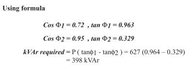
Using table (see Table 1.2)
1) Locate 0.72 (original power factor) in column (1).
2) Read across desired power factor to 0.95 column. We find 0.635 multiplier
3) Multiply 627 (average kW) by 0.635 = 398 kVAr.
4) Install 400 kVAr to improve power factor to 95%.

Location of Capacitors
The primary purpose of capacitors is to reduce the maximum demand. Additional benefits are derived
by capacitor location. The Figure 1.13 indicates typical capacitor locations. Maximum benefit of
capacitors is derived by locating them as close as possible to the load. At this location, its kilovars are
confined to the smallest possible segment, decreasing the load current. This, in turn, will reduce power
losses of the system substantially. Power losses are proportional to the square of the current. When
power losses are reduced, voltage at the motor increases; thus, motor performance also increases.

Capacitor correction is relatively inexpensive both in material and installation costs. Capacitors can
be installed at any point in the electrical system, and will improve the power factor between the point
of application and the power source. However, the power factor between the utilization equipment and
the capacitor will remain unchanged. Capacitors are usually added at each piece of offending equipment,
ahead of groups of small motors (ahead of motor control centers or distribution panels) or at main
services.
The advantages and disadvantages of each type of capacitor installation are listed below:
Capacitor on each piece of equipment (1,2)
Advantages
o Increases load capabilities of distribution system.
o Can be switched with equipment; no additional switching is required.
o Better voltage regulation because capacitor use follows load.
o Capacitor sizing is simplified.
o Capacitors are coupled with equipment and move with equipment if rearrangements are
instituted.
Disadvantages
o Small capacitors cost more per kVAr than larger units (economic break point for individual
correction is generally at 10 HP).
It should be noted that the rating of the capacitor should not be greater than the no-load magnetizing
kVAr of the motor. If this condition exists, damaging over voltage or transient torques can occur. This
is why most motor manufacturers specify maximum capacitor ratings to be applied to specific motors.
Capacitor with equipment group (3)
Advantages
o Increased load capabilities of the service
o Reduced material costs relative to individual correction
o Reduced installation costs relative to individual correction
Disadvantages
o Switching means may be required to control amount of capacitance used.
The advantage of locating capacitors at power centers or feeders is that they can be grouped together.
When several motors are running intermittently, the capacitors are permitted to be on line all the time,
reducing the kVA demand regardless of load.
Capacitor at main service (4,5, & 6)
Advantages
o Low material installation costs.
Disadvantages
o Switching will usually be required to control the amount of capacitance used.
oDoes not improve the load capabilities of the distribution system.
From energy efficiency point of view, capacitor location at receiving substation only helps the utility
in loss reduction. Locating capacitors at tail end will help to reduce loss reduction within the plants
distribution network as well and directly benefit the user by reduced consumption. Reduction in the
distribution loss% in kWh when tail end power factor is raised from PF, to a new power factor PF2 will be proportional to

Other Considerations
Where the loads contributing to power factor are relatively constant, and system load capabilities are not
a factor, correcting at the main service could provide a cost advantage. When the low power factor is
derived from a few selected pieces of equipment, individual equipment correction would be cost effective.
The growing use of ASDs (nonlinear loads) has increased the complexity of system power factor and
its corrections. The application of PF correction capacitors without a thorough analysis of the system
can aggravate rather than correct the problem, particularly if the fifth and seventh harmonics are present.
Capacitors for Other Loads
The other types of load requiring capacitor application include induction furnaces, induction heaters
and arc welding transformers etc. The capacitors are normally supplied with control gear for the
application of induction furnaces and induction heating furnaces. The PF of arc furnaces experiences
a wide variation over melting cycle as it changes from 0.7 at starting to 0.9 at the end of the cycle.
Power factor for welding transformers is corrected by connecting capacitors across the primary winding
of the transformers, as the normal PF would be in the range of 0.35.
Performance Assessment of Power Factor Capacitors
Voltage effects: Ideally capacitor voltage rating is to match the supply voltage. If the supply voltage
is lower, the reactive kVAr produced will be the ratio V,2 /V,2 where V, is the actual supply voltage,
V, is the rated voltage.
On the other hand, if the supply voltage exceeds rated voltage, the life of the capacitor is adversely
affected.
Material of capacitors:
Power factor capacitors are available in various types by dielectric material
used as; paper/ polypropylene etc. The watt loss per kVAr as well as life vary with respect to the choice
of the dielectric material and hence is a factor to be considered while selection.
Connections:
Shunt capacitor connections are adopted for almost all industry/ end user applications,
while series capacitors are adopted for voltage boosting in distribution networks.
Operational performance of capacitors:
This can be made by monitoring capacitor charging current
vis- a- vis the rated charging current. Capacity of fused elements can be replenished as per requirements.
Portable analyzers can be used for measuring kVAr delivered as well as charging current. Capacitors
consume 0.2 to 6.0 Watt per kVAr, which is negligible in comparison to benefits.
Some checks that need to be adopted in use of capacitors are:
i. Nameplates can be misleading with respect to ratings. It is good to check by charging
currents.
ii. Capacitor boxes may contain only insulated compound and insulated terminals with no
capacitor elements inside.
iii. Capacitors for single phase motor starting and those used for lighting circuits for voltage
boost, are not power factor capacitor units and these cannot withstand power system
conditions.
Transformers
A transformer can accept energy at one voltage and deliver it at
another voltage. This permits electrical energy to be generated
at relatively low voltages and transmitted at high voltages and
low currents, thus reducing line losses and voltage drop (see
Figure 1.14).
Transformers consist of two or more coils that are electrically
insulated, but magnetically linked. The primary coil is connected
to the power source and the secondary coil connects to the load. The turn’s ratio is the ratio between the numbers of turns on the secondary to the turns on the primary (See Figure 1.15).
The secondary voltage is equal to the primary voltage times the turn’s ratio. Ampere-turns are calculated by multiplying the
current in the coil times the number of turns. Primary ampere- turns are equal to secondary ampere-turns. Voltage regulation of a transformer is the percent increase in voltage from full load to no load.

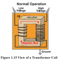
Types of Transformers
Figure 1.15 View of a Transformer Coil
Transformers are classified as two categories: power transformers and distribution transformers.
Power transformers are used in transmission network of higher voltages, deployed for step-up and step
down transformer application (400 kV, 200 kV, 110 kV, 66 kV, 33kV)
Distribution transformers are used for lower voltage distribution networks as a means to end user
connectivity. (11kV, 6.6 kV, 3.3 kV, 440V, 230V)
Rating of Transformer
Rating of the transformer is calculated based on the connected load and applying the diversity factor
on the connected load, applicable to the particular industry and arrive at the kVA rating of the
Transformer. Diversity factor is defined as the ratio of overall maximum demand of the plant to the
sum of individual maximum demand of various equipment. Diversity factor varies from industry to
industry and depends on various factors such as individual loads, load factor and future expansion
needs of the plant. Diversity factor will always be less than one.
Location of Transformer
Location of the transformer is very important as far as distribution loss is concerned. Transformer
receives HT voltage from the grid and steps it down to the required voltage. Transformers should be
placed close to the load centre, considering other features like optimization needs for centralized
control, operational flexibility etc. This will bring down the distribution loss in cables.
Transformer Losses and Efficiency
The efficiency varies anywhere between 96 to 99 percent. The efficiency of the transformers not only
depends on the design, but also, on the effective operating load.
Transformer losses consist of two parts: No-load loss and Load loss
1.No-load loss (also called core loss) is the power consumed to sustain the magnetic field in
the transformer’s steel core. Core loss occurs whenever the transformer is energized; core
loss does not vary with load. Core losses are caused by two factors: hysteresis and eddy
current losses. Hysteresis loss is that energy lost by reversing the magnetic field in the core
as the magnetizing AC rises and falls and reverses direction. Eddy current loss is a result of
induced currents circulating in the core.
2. Load loss (also called copper loss) is associated with full-load current flow in the transformer
windings. Copper loss is power lost in the primary and secondary windings of a transformer
due to the ohmic resistance of the windings. Copper loss varies with the square of the load
current. (P=I’R). Typical 3 Phase Transformer losses of various capacities is given in Table1.3.
Transformer losses as a percentage of load is given in the Figure 1.16.

For a given transformer, the manufacturer can supply values for no-load loss, P no load & load loss PLOAd .The total transformer loss, P
TOTAL at any load level can then be calculated from:


Voltage Fluctuation Control
A control of voltage in a transformer is important due to frequent changes in supply voltage level.
Whenever the supply voltage is less than the optimal value, there is a chance of nuisance tripping of
voltage sensitive devices. The voltage regulation in transformers is done by altering the voltage
transformation ratio with the help of tapping.
There are two methods of tap changing facility available: Off-circuit tap changer and On-load tap
changer.
Off-circuit tap changer
It is a device fitted in the transformer, which is used to vary the voltage transformation ratio. Here the
voltage levels can be varied only after isolating the primary voltage of the transformer.
On load tap changer (OLTC)
The voltage levels can be varied without isolating the connected load to the transformer. To minimize
the magnetization losses and to reduce the nuisance tripping of the plant, the main transformer (the
transformer that receives supply from the grid) should be provided with On Load Tap Changing facility
at design stage. The downstream distribution transformers can be provided with off-circuit tap changer.
The On-load gear can be put in auto mode or manually depending on the requirement. OLTC can be arranged for transformers of size 250 kVA onwards. However, the necessity of OLTC below 1000 kVA can be considered after calculating the cost economics.
The On-load gear can be put in auto mode or manually depending on the requirement. OLTC can be arranged for transformers of size 250 kVA onwards. However, the necessity of OLTC below 1000 kVA can be considered after calculating the cost economics.
Parallel Operation of Transformers
The design of Power Control Centre (PCC) and Motor Control Centre (MCC) of any new plant should
have the provision of operating two or more transformers in parallel. Additional switchgears and bus
couplers should be provided at design stage.
Whenever two transformers are operating in parallel, both should be technically identical in all aspects
and more importantly should have the same impedance level. This will minimize the circulating current
between transformers.
Where the load is fluctuating in nature, it is preferable to have more than one transformer running in
parallel, so that the load can be optimized by sharing the load between transformers.
The transformers
can be operated close to the maximum efficiency range by this operation.
For operating transformers in parallel, the transformers should have the following principal
characteristics.
° The same phase angle difference between the primary and secondary terminals.
° Same voltage ratio
° Same percentage impedance
° Same polarity
° Same phase sequence
Energy Efficient Transformers
Most energy loss in dry-type transformers occurs through heat or vibration from the core. The new
high-efficiency transformers minimize these losses. The conventional transformer is made up of a
silicon alloyed iron (grain oriented) core. The iron loss of any transformer depends on the type of core
used in the transformer. However the latest technology is to use amorphous material — a metallic glass
alloy for the core (see Figure 1.17). The expected reduction in core loss over conventional (Si Fe core)
transformers is roughly around 70%, which is quite
significant. By using an amorphous core— with
unique physical and magnetic properties- these new
types of transformers have increased efficiency even
at low loads - 98.5% efficiency at 35% load.

Standards & Labeling Programme for Distribution Transformers
The Bureau of Energy Efficiency has included Distribution transformers under Standards & Labeling
Programme as large number of Distribution transformers are used by Electricity supply companies
and also by different users for supplying power to their load centers.
This provision has been made
mandatory with effect from 7" January 2010.
The existing efficiency or the loss standards are specified in IS 1180 (part 1). This standard defines
load losses and no load losses separately.
For the BEE labeling programme total losses at 50% and
100% load have been defined. The highest loss segment is defined as star 1 and lowest loss segment
is defined as star 5. The existing IS 1180 (part 1) specification losses are the base case with star 1.
The details of Star Rating plan for Distribution transformers and corresponding losses are given in
Table 1.4. More details can be obtained from www.beestarlabel.com.

In an electrical system often the constant no load losses and the variable load losses are to be assessed,
over long reference duration, for energy loss estimation.
Identifying and calculating the sum of the individual contributing loss components is a challenging
one, requiring extensive experience and knowledge of all the factors impacting the operating efficiencies
of each of these components.
For example the cable losses in any industrial plant will be up to 6 percent depending on the size and
complexity of the distribution system. All of these are current dependent, and can be readily mitigated
by any technique that reduces facility current load. The various losses in different distribution
equipments are given in Table1.5.
In system distribution loss optimization, the various options available include:
° Relocating transformers and sub-stations near to load centers
° Relocating transformers and sub-stations near to load centers
° Re-routing and re-conducting such feeders and lines where the losses / voltage drops are higher.
° Power factor improvement by incorporating capacitors at load end.
° Optimum loading of transformers in the system.
° Opting for lower resistance All Aluminum Alloy Conductors (AAAC) in place of conventional
Aluminum Cored Steel Reinforced (ACSR) lines
° Minimizing losses due to weak links in distribution network such as jumpers, loose contacts,
and old brittle conductors.

Assessment of Transmission and Distribution (T&D) Losses in Power Systems
For an electric utility (DISCOMs) the distribution losses which are more predominant, can be
categorized as
1) Technical Losses
ii) Commercial Losses
Technical Losses:
The technical losses primarily take place due to the following factors
o Transformation Losses (at various transformation levels)
o High IR losses in distribution lines due to inherent resistance and poor power factor in the
electrical network
Normative Technical loss limits in Indian Transmission and Distribution network are shown in Table 1.6.

The first and important step in reduction of energy losses is to carry out energy audit of power distribution
system. There are two methods of determining the energy losses namely direct method and indirect
method.
The Direct method involves placement of energy meters at all locations starting from the input point
of the feeder to the individual consumers. The difference between input energy and sum of all consumers
over a specific duration is accounted as distribution loss of the network. This calls for elaborate and
accurate metering and collection of simultaneous data.
The Indirect method essentially involves:
° Energy metering at critical locations in the system such as substation and feeders.
° Compiling the network information, such as length of the line/feeders, conductor size, DTR
details, capacitor details etc.
° Conducting load flow studies (all electrical parameters) on peak load durations as well as normal
load durations.
° Application of suitable software to assess the system losses.
This software can also be used for system simulation, identifying improvements and network
optimization.
Causes of technical losses in distribution system
The factors contributing to the increase in the distribution losses are
1. Lengthy distribution lines:
In practice, 11 KV and 415 volts lines, in rural areas are extended radially over long distances to feed
loads scattered over large areas. This results in high line resistance and therefore high I’R losses in the
line.
2. Inadequate Size of Conductors:
On account of load growth, many distribution feeders end up being under sized for the loads to be
catered to the consumers. The size of the conductors should be selected/upgraded/transformers to be
relocated on the basis of KVA Kilometer capacity of standard conductor to maintain voltage regulation
within limits.
Voltage Regulation:
The voltage regulation is usually expressed as a percentage drop with reference to the receiving end
voltage.
Percentage regulation = 100 (Es - Er) / Er
Where, Es = Sending end voltage
Er = Receiving end voltage
3. Distribution Transformers (DTR) not located at load center on the Secondary Distribution
System:
Often, DTs are not located centrally with respect to consumer loads. Consequently, the farthest
consumers receive low voltage even though a good voltage level is maintained at the transformer’s
secondary. This again leads to high line loss. Therefore in order to reduce the voltage drop in the line
to the farthest consumers, the distribution transformer should be located near to consumer load to keep
voltage drop within permissible limits.
4. Low Power Factor:
A low PF contributes towards high distribution losses. For a given load, if the PF is low, the current
drawn is high. Consequently, the losses which are proportional to square of the current will be more.
Therefore, line losses owing to the poor PF can be reduced by improving the PF. This can be done by
application of shunt capacitors.
Shunt capacitors can be connected in the following locations:
o On the secondary side (11 KV side) of the 33/11 KV power transformers in substation.
o On the secondary side of distribution transformers
The following example shows how the improvement in power factor in 11 KV lines results in
considerable reduction in losses:

Some of the measures to reduce technical losses in distribution system include,
o High Voltage Distribution System (HVDS):- Distribution Companies (Discoms) have started
implementing distribution systems at high voltage. The L.T. distributions are reduced and
eliminated wherever feasible. A typical LT System consists of LT 3 Phase 415V Distribution
System with lengthy LT Lines serving the consumers, contributing to more losses in the
System. Reduction in these losses is done through restructuring of the existing LVDS network
to HVDS network by installation of three phase 11 kV/400V 25 KVA & 16K VA pole mounted
transformers at the load centers to serve different consumers.
o Amorphous Core Transformers: Recently Distribution Transformers DTRs with amorphous
core have been manufactured with just about 30% of no-load losses compared to the Conventional
Transformers. Some of the Discoms have installed these transformers to reduce the distribution
loess in the network.
Commercial Losses
Any illegal consumption of electrical energy, which is not correctly metered, billed and revenue
collected, causes commercial losses to the utilities. The commercial losses are primarily attributable
to discrepancies in:
Meter Reading: Commercial losses occur due to discrepancy in meter reading. Meter reading problems
are manifested in the form of zero consumption in meter reading books which may be due to premises
found locked, untraceable consumers, stopped/defective meters, temporarily disconnected consumers
continuing in billing solution etc. Collusion with consumers is also a source of commercial loss to
utilities which are primarily due to incorrect meter reading.
Metering: Most utilities use either electro-mechanical or electronic meters for consumer metering.
Commercial losses through metering can be in the form of meter tampering in various forms.
Collection efficiency: Typically in a billing cycle, a distribution utility issues bills against metered
energy and assessed (generally in case of agricultural loads and temporary connections) energy. The
ratio of amount collected to total amount billed is termed as collection efficiency.
The above losses are collectively categorized as AT & C (Aggregate Technical & Commercial) losses.
The estimation of AT & C losses for a sample area is shown in Table 1.7.
Computation of AT & C Losses
The aggregate technical and commercial losses can be measured using the formula mentioned below.
AT & C Losses = {1- (Billing Efficiency x Collection Efficiency)} x 100
Where,

Measures to Reduce Commercial Losses
Some of the measures to reduce commercial losses in distribution system include:
° Accurate Metering (A metering plan for installing meters with sustained accuracy).
° Appropriate range of meter with reference to connected load.
° Installation of Electronic meters with (TOD, tamper proof, data and remote reading facility).
° Intensive inspections.
° Compulsory metering/average billing
° Use of energy audit as a tool to pinpoint areas of high losses.
° Eradication of theft.
Demand Side Management (DSM)
DSM refers to “Actions taken on the customer’s side of the meter to change the amount (kWh) or
timing (kVA) of energy consumption. Electricity DSM strategies have the goal of maximizing end use
efficiency to avoid or postpone the construction of new generating plants”.
The ever increasing demand growth of electricity can be met either by matching increase in capacity,
i.e. Supply side capacity addition or adopting demand side management and end use efficiency
improvement strategies, which are much more cost effective and resource efficient.
Utilities are driven by supply side and customer side concerns such as capacity (peak demand) short falls,
energy shortfalls, need for optimization of generation and network utilization, Regulatory issues,
environmental mandates and customer demand for uninterrupted supply at competitive tariffs. Demand
side management offers itself as a powerful tool to distribution companies, to analyze, develop and implement
customized DSM programs, cost effectively, to enable meeting the supply side concern of the utilities.
DSM Objectives
The key objectives of DSM include the following.
¢ Improve the efficiency of energy systems.
¢ Reduce financial needs to build new energy facilities (generation).
¢ Minimize adverse environmental impacts.
¢ Lower the cost of delivered energy to consumers.
¢ Reduce power shortages and power cuts.
¢ Improve the reliability and quality of power supply.
DSM methodology
Step 1: Load Research
This stage in the DSM implementation will typically assess the customer base, tariff, load profile on
an hourly basis and will identify the sectors contributing to the load shape. This step will also identify
peak load contributors.
Step 2: Define load-shape objectives
Based on the results of the load research in the utility, the load shape objectives for the current situation
are defined. Various load-shape objectives are represented in Figure 1.18 below.

Meaning of load-shape objective
Peak Clipping: the reduction of utility load primarily during periods of peak demand.
Valley-Filling: the improvement of system load factor by building load in off-peak periods.
Load Shifting: the reduction of utility loads during periods of peak demand, while at the same time
building load in off-peak periods. Load shifting typically does not substantially alter total electricity
sales.
Conservation: the reduction of utility loads, more or less equally, during all or most hours of the day.
Load Building: the increase of utility loads, more or less equally, during all or most hours of the day.
Flexible Utility Load Shape: refers to programs that set up utility options to alter customer energy
consumption on an as-needed basis, as in interruptible/ curtailable agreements.
Step 3: Assess program implementation strategies
This step will identify the end-use applications that can be potentially targeted to reduce peak demand,
specifically in sectors contributing to system peak. This step will also carry out a detailed cost benefit
analysis for the end-users and the utilities, including analysis of societal as well as environmental
benefits.
Step 4: Implementation
Implementation stage includes program design for specific end-use applications, promotes the program
to the target audience through marketing approaches such as advertising, bills and inserts, and focused
group meetings (specifically in case of commercial and industrial sector).
Step 5: Monitoring and Evaluation
This step tracks the program design and implementation and compares the same with proposed DSM
goal set by the utility. A detailed benefit-cost analysis in this case includes identifying the avoided
supply cost for the utility vis-a-vis the total program cost for the utilities and benefits to the participants
including the reduced bills or incentives to the end-users.
Types of DSM Measures
Broadly the types of DSM measures can be classified as follows.
a) Energy reduction programmes - reducing demand through more efficient processes, buildings or
equipment, for example:
Efficient Lighting (CFLs, Using natural light), Appliance Labelling, Building regulations, Efficient
and alternative energy use, Efficient use of electric motors and motor driven systems, Preventative
maintenance, Energy management and audit.
b) Load management programmes - changing the load pattern and encouraging less demand at peak
times and peak rates, for example:
Load Levelling (Peak clipping, Valley filling and load shifting), Load growth, Tariff Incentives or
Penalties (Time-of-Use & real time pricing, power factor penalties)
Benefits of DSM
Benefits of the DSM initiatives are manifold, some of which are described in Table 1.8 below.

Harmonics
A harmonic is a component frequency of the signal that is an integer multiple of the fundamental
frequency. Harmonic voltages and currents in an electric power system are a result of non-linear electric
loads. The Harmonic current represents energy that cannot be used by any devices on the network.
It will be therefore converted to heat and is wasted. For instance, the fundamental frequency is 50
Hz, and then the 5th harmonic is five times that frequency, or 250 Hz (Figure 1.19).

Linear System
In any alternating current network, flow of current depends upon the voltage applied and the impedance
(resistance to AC) provided by elements like resistances, reactances of inductive and capacitive nature.
As the value of impedance in above devices is constant, they are called linear whereby the voltage and
current relation is of linear nature.
e.g. Incandescent lamps, heaters and, to a great extent, motors are linear systems.
Non-linear System
Non-Linear systems are one with varying impedance characteristics, These NON LINEAR devices
cause distortion in voltage and current waveforms which is of increasing concern in recent times.
e.g. Variable frequency drives (VFDs), electronic ballasts, UPS and Computers, induction and arc
furnaces
Current Distortion:
Current Harmonics could cause transformer heating or nuisance tripping by fuses, circuit breakers and
other protective devices since they are typically not rated for harmonically rich waveforms.

A 5th harmonic current is simply a current flowing at 250 Hz on a 50 Hz system. The 5th harmonic current
flowing through the system impedance creates a 5th harmonic voltage. Total Harmonic Distortion (THD)
expresses the amount of harmonics. The following is the formula for calculating the THD for current:

Current at fundamental frequency I, = Base Current = 250 amps
Third Harmonic current = 50 amps
Fifth Harmonic current = 35 amps
When harmonic currents flow in a power system, they are known as “poor power quality” or “dirty
power’. Other causes of poor power quality include transients such as voltage spikes, surges, sags,
and ringing. Because they repeat every cycle, harmonics are regarded as a steady-state cause of poor
power quality. The distortion travels back into the power source and can affect other equipment
connected to the same source.
Voltage Distortion:
A distorted current has higher peak values that cause non-sinusoidal voltage drops across the distribution
system. The resulting voltage drops add or subtract from the sinusoidal voltage supplied by the utility.
Other utility customers could get distorted voltage on the downstream side of the power distribution
circuit.
When expressed as a percentage of fundamental voltage THD is given by,

Harmonic currents and voltages are created by non- linear loads connected to the power distribution
system. All power electronic converters used in different types of electronic systems can increase
harmonic disturbances by injecting harmonic currents directly into the supply network. Common nonlinear loads include variable speed drives (AC as well as DC), induction furnaces, LED based and
CFL lamps, certain types of UPS & computer power supplies.
Effects of Harmonics
o Blinking of Incandescent Lights - Transformer Saturation
o Capacitor Failure - Harmonic Resonance
o Circuit Breakers Tripping - Inductive Heating and Overload
o Conductor Failure - Inductive Heating
o Electronic Equipment Shutting down - Voltage Distortion
o Flickering of Fluorescent Lights - Transformer Saturation
o Fuses Blowing for No Apparent Reason - Inductive Heating and Overload
o Motor Failures (overheating) - Voltage Drop
o Neutral Conductor and Terminal Failures - Additive Triplen Currents
o Electromagnetic Load Failures - Inductive Heating
o Overheating of Metal Enclosures - Inductive Heating
o Power Interference on Voice Communication - Harmonic Noise
o Transformer Failures - Inductive Heating
Overcoming Harmonics in Power systems
Passive Filters: Built-up by combinations of capacitors, inductors (reactors) and resistors. It is the
most common and available for all voltage levels
Active Power Filter APF: Inserting negative phase compensating harmonics into the AC-Network,
thus eliminating the undesirable harmonics on the AC power network.
Special Transformers: There are several special types of transformer connections which can cancel
harmonics. Additional special winding connections can be used to cancel other harmonics on balanced
loads. These systems also use more copper. Harmonic canceling transformers are also known as phase shifting transformers. It is a relatively new power quality product for mitigating harmonic problems.
Since VFD is emerging as a major energy saving application and results in harmonic generation,
harmonic mitigation in VFD is discussed here.
The Harmonic Mitigation solutions currently in use in the industry broadly fall into the following
categories:
1. Passive Harmonic Filter (PHF)
2. Advance Active Filters (AAF)
3. Active Front End based VFDs (AFE)
They are briefly described in the sections below:
Passive filter is the most common method for the cancellation of harmonic current in the distributed
system. These filters are basically designed on principle either single tuned/double tuned or band pass
filter technology. Passive filters (Figure 1.20) offer very low impedance in the network at the tuned
frequency to divert all the harmonic current at the tuned frequency.

Active filter is connected parallel with the distribution system. Distribution system consists of a wide
percentage of harmonics produced by non- linear loads. Active filters (Figure 1.21) compensate current
harmonics by injecting equal magnitude but opposite phase harmonic compensating current.

Active Front end Rectifiers used in VFDs has the major advantage of mitigation of harmonics without
using external filter, to maintain unity power factor at the point of common coupling, Bidirectional
power flow makes recovery of energy to the mains by saving it, Clean power to the grid which in turn
does not affect the other loads connected to it, maintaining the DC voltage irrespective of the supply
variations.
LCL Filter is connected at Point of Common Coupling (PCC) between Grid and active Front End
Rectifier (AFE) (Figure 1.22). Due to High switching frequency operation of AFE IGBTs there will
be harmonics in the Sinusoidal waveform at that particular High frequency. The LCL (Inductance and
Capacitance Combination) is introduced to bypass those Switching frequencies which will in turn have
approximately sinusoidal supply at the Grid.

Current Distortion Limits for General Distribution System’s end-User limits (120 Volts To 69,000
Volts) 


Note:
High voltage systems can have up to 2.0% THD where the cause is an HVDC terminal that will
attenuate by the time it is tapped for a user.
Two very important points must be made in reference to the above.
1. The customer is responsible for maintaining current distortion to within acceptable levels, while
the utility is responsible for limiting voltage distortion.
2. The limits are only applicable at the point of common coupling (PCC) between the utility and
the customer. The PCC, while not explicitly defined, is usually regarded as the point at which
the utility equipment ownership meets the customer’s or the metering point.
Therefore, the above limits cannot be meaningfully applied to distribution panels or individual
equipment within a plant. The entire plant must be considered complying with these limits.
Analysis of Electrical Power Systems
An analysis of an electrical power system may uncover energy waste, fire hazards, and equipment
failure. Facility /energy managers increasingly find that reliability-centered maintenance can save
money, energy, and downtime (see Table 1.11).
Table 1.11 Trouble shooting of Electrical Power Systems

Solved Example:
An energy audit of electricity bills of a process plant was conducted. The plant has a contract demand
of 5000 kVA with the power supply company. The average maximum demand of the plant is 3850 kVA/
month at a power factor of 0.95. The maximum demand is billed at the rate of Rs.600/kVA/month. The
minimum billable maximum demand is 75 % of the contract demand. An incentive of 0.5 % reduction
in energy charges component of electricity bill are provided for every 0.01 increase in power factor
over and above 0.95. The average energy charge component of the electricity bill per month for the
plant is Rs.18 lakhs.
The plant decides to improve the power factor to unity. Determine the power factor capacitor kVAr
required, annual reduction in maximum demand charges and energy charge component. What will be
the simple payback period if the cost of power factor capacitors is Rs.900/kVAr.

-------------------------
Comments
Post a Comment