Energy efficiency in Thermal utilities (Chapter 9: Heat Exchanger)

Energy efficiency in Thermal utilities 

(Chapter 9: Heat Exchanger)

Heat Transfer Basics Heat transfer is the transition of thermal energy from a hotter object to a cooler object. 

Heat flows from a hot or warm medium to a cold medium in three ways: 

o By radiation from a warm surface to a cooler surface through air space 

 o By conduction through solid or fluid materials 

 o By convection which involves the physical movement of air  

Criteria for heat transfer are 

o Difference in temperature between the hot and cold fluids, greater the difference- higher the rate at which the heat will flow between them.

o Area of the conductive barrier provided for heat flow. The greater the area, the larger the amount of heat that will flow in a given time with a given temperature difference.

o Rate of heat flow into, or, out, from each of the fluids. High resistance to heat flow in either fluid will produce a slow overall rate of transfer. 

o Flow of heat through the conductive barrier between fluids. Material chosen has to be compatible with the fluids of the process, it must not corrode or contaminate the fluids.  

Concept of Heat Exchangers 

A heat exchanger is a device which allows transfer of heat energy from one fluid to another fluid, generally without mixing the two different fluids. Regardless of the function that a heat exchanger fulfills, to transfer heat, the fluids involved must be at different temperatures and they must come into thermal contact, since heat can flow only from the hotter to the cooler fluid. 

A heat exchanger can serve any of the following purposes 

1.To heat a cooler fluid by means of a hotter fluid 

2. To reduce the temperature of a hot fluid by means of a cooler fluid 

3. To boil a liquid by means of a hotter fluid 

4. To condense a gaseous fluid by means of a cooler fluid 

5.To boil a liquid while condensing a hotter gaseous fluid 

Heat Exchanger Theory 

 The heat gained or lost by a fluid in a heat exchanger is given by the following formula: 

 Q=mxCpxAT

Where, 

Q = heat transferred (kW)

m = mass flow of the fluid (kg/s) 

Cp= specific heat of the fluid (kJ/kg/°C) 

ΔT= Temperature difference between inlet and outlet of a fluid (°C) 

The basic concept of a heat exchanger is based on the principle that the loss of heat on the high temperature side is exactly the same as the heat gained by the low temperature side. This is expressed by the following formula: 

Where subscript “h” = hot fluid, subscript “c” = cold fluid 

In theory, the heat given up by the hot fluid is never exactly equal to the heat gained by the cold fluid due to environmental heat losses. However, in practice they are generally assumed to be equal to simplify the calculations involved. Any environmental losses that occur are generally minimized with insulation of equipment and piping. 

Example : Calculate the mass flow rate of cooling water required for the heat exchanger shown in figure with the following data:

Mass flow rate of process fluid — 1000 kg/hr Specific heat of process fluid — 0.9 keal/kg°C Specific heat of water — 1 kcal/kg°C 

The Heat Exchanger Design Equation 

Heat exchanger theory leads to the basic heat exchanger design equation as follows: 

Where, 

Q is the rate of heat transfer between the two fluids in the heat exchanger in kceal/hr or kJ/hr 

U is the overall heat transfer coefficient in kcal/hr m2°C or W/m2K.

A is the heat transfer surface area in m’, and AT, 

the log mean temperature difference in °C, calculated from the inlet and outlet temperatures of both fluids as follows.     

For design of heat exchangers, the basic heat exchanger design equation can be used to calculate the required heat exchanger area for known or estimated values of the other three parameters, Q, U, and The assumptions that are made in its derivation are that the overall heat transfer coefficient and the specific heat of the fluids remain constant through the heat exchanger.

Log Mean Temperature Difference

The driving force for any heat transfer process is the temperature difference between two fluids. In  the heat transfer process, the temperatures of the two fluids keep changing as they pass through the heat exchanger, for which some type of average temperature difference is needed. This average temperature difference through the heat exchanger is described by the log mean temperature difference (LMTD) (Refer Figure 9.2). The larger the temperature difference, the smaller the required heat exchanger area and vice versa.

In Figure 9.1 it appears that the temperature difference between the fluids remains almost constant throughout the heat exchanger. This is rarely the case. In the Figure 9.2 a process stream at 94°C is to be cooled to 65°C using cooling water available at 30°C. It can be observed from the TQ diagram that the temperature difference between the two streams vary widely. This is why the log mean temperature difference is used. In this example the LMTD can be calculated as: 

   

There can be special cases where the LMTD equation shown above is not applicable. Consider the case in Figure 9.3. If the LMTD equation is applied to this special case the result would be zero. In this case the LMTD is the same as the temperature difference on each LMTD is the same as the temperature difference on each Difference), or 30°C.    

Overall Heat Transfer Coefficient, U 

The overall heat transfer coefficient describes the rate of heat transfer in the heat exchanger. The overall heat transfer coefficient is a calculated variable based on the physical properties of the fluids involved in the heat transfer (hot and cold) as well as the geometry and type of heat exchanger to be used. 
The overall heat transfer coefficient, U, depends on the conductivity through the heat transfer wall separating the two fluids, and the convection coefficients on both sides of the heat transfer wall. Typically in a shell and tube heat exchanger, there would be an inside convective coefficient for the tube side fluid and an outside convective coefficient for the shell side fluid. Generically, it is described by the following equation:

The heat transfer coefficient for a given heat exchanger is often determined empirically by measuring all of the other parameters in the basic heat exchanger equation and calculating U.

The Temperature Correction Factor, F 

The temperature correction factor, F, is used to correct the log mean temperature difference for heat exchangers that lack truly counter-current flow. Many different heat transfer technologies lack truly counter-current flow patterns as a result of their inherent mechanical design. Generally, the value of F lies between 0.85 and 0.98. There are cases when this value can be taken as one, but only if the flow in the exchanger is purely counter-current. The charts are available to look up the temperature correction factor for a given configuration.  

Heat Exchanger Types (by flow design) 

The flow pattern of the two fluids in a heat exchanger can vary depending on the heat exchanger design and type. Typically the process conditions, available space and economics will define the type and configuration of the heat exchanger. According to the type of flow pattern heat exchangers can be broadly classified as counter flow, parallel flow and cross flow. 

Counterflow:

The most effective configuration from a heat transfer standpoint is a counter flow design (also called counter current). In a counter flow arrangement the hot fluid and cold fluid move in opposite directions (Refer Figure 9.4 & 9.5), such that, at one terminal point; the hot side inlet temperature (hottest) is in contact with the cold side outlet temperature (hottest) and at the other terminal point; the cold side inlet temperature (coldest) is in contact with the hot side outlet temperature (coldest). Counter flow designs are most valuable when there is a temperature cross. A temperature cross occurs when the desired outlet temperature of one fluid is between the inlet and outlet temperatures of the other fluid. A true counter flow design is difficult to achieve or impractical for many common heat exchanger applications. However, close to true counter flow could be obtained using plate heat exchangers, double pipe exchangers and spiral heat exchangers.

Where, ΔT1 and ΔT2 are the temperature differences at the two terminal points. 
 

Parallel flow 

The reverse configuration to counter flow would be parallel flow, where the hot fluid and cold fluid move in the same direction (Figure 9.6 & 9.7), such that, at one terminal point; the hot side inlet temperature (hottest) is in contact with the cold side inlet temperature (coldest), the two fluid progress through the heat exchanger and at the other terminal point; the cold side outlet temperature (hottest) is in contact with the hot side outlet temperature (coldest). A temperature cross cannot be achieved with a parallel flow exchanger. Parallel flow configuration is frequently used in applications where it is desired that the two fluids have close to the same exiting temperatures.  

Where, ΔT, and ΔT, are the temperature differences at the two terminal points.  

Cross flow 

Most shell and tube heat exchangers and air-cooled heat exchangers are of cross flow design because it can sometimes be impractical to use a counter flow design due to high flow volumes or space restrictions. The flow patterns of two fluids in a cross flow heat exchanger are at right angles to each other (Figure 9.8). In most applications, at least one fluid makes multiple passes so there is a combination of cross flow and counter flow occurring. With the thermal advantage gained from a multi-pass configuration a temperature cross can be produced in cross flow heat exchanger but not to the same degree as in a true counter flow configuration.

Heat Exchanger Types (by construction) 

Double Pipe heat Exchangers 

The double pipe heat exchanger is probably one of the simplest configurations found in applications.It consists of two concentric circular tubes with one fluid flowing inside the inner tube and the other fluid flowing inside the annular space between the tubes as shown in figure 9.9. Its primary uses are in cooling process fluids where small heat transfer areas are required. It may be designed in a number of arrangements such as parallel flow and counter flow, and combined in series or parallel arrangements with other heat exchangers to form a system. 

Shell and Tube heat Exchangers 

Shell-and-tube heat exchangers (Figures 9.10) consist of a bundle of parallel tubes that provide the heat-transfer surface separating the two fluid streams. The tube-side fluid passes axially through the inside of the tubes; the shell-side fluid passes over  the outside of the tubes. Baffles external and perpendicular to the tubes direct the flow across the tubes and provide tube support. 

Tube sheets seal the ends of the tubes, ensuring separation of the two streams. The process fluid is usually placed inside the tubes for ease of cleaning or to take advantage of the higher pressure capability inside the tubes. The thermal performance of such an exchanger usually surpasses a coil type but is less than a plate type. Pressure capability of shell-and-tube exchangers is generally higher than a plate type but lower than a coil type. 

Plate Heat Exchangers 

Plate heat exchangers (Figure 9.11) consist of a stack of parallel thin plates that lie between heavy end plates. Each fluid stream passes alternately between adjoining plates in the stack, exchanging heat through the plates. The plates are corrugated for strength and to enhance heat transfer by directing the flow and increasing turbulence. These exchangers have high heat-transfer coefficients and area, the pressure drop is also typically low, and they often provide very high effectiveness. However, they have relatively low pressure capability. 

Perhaps the biggest advantage of the plate and frame heat exchanger, and a situation where it is most often used, is when the heat transfer application calls for the cold side fluid to exit the exchanger at a temperature significantly higher than the hot side fluid exit temperature. This situation is best explained with another set of T-Q diagrams.

Duty 1 shown in the Figure 9.12 (A) can be easily accomplished in a simple shell and tube heat exchanger.

Duty 2 shown in the Figure 9.12 (B) has a severe “temperature cross” or the cold side fluid exiting higher than the hot side fluid. This would require several shell and tube exchangers in series due to the lack of purely counter-current flow. On the other hand, this duty is easily accomplished in a single plate and frame heat exchanger. 

The overall heat transfer coefficient of plate heat exchangers under favorable circumstances can be as high as 8,000 W/m?°C. With traditional shell and tube heat exchangers, the U-value will be below 2,500 W/m2 °C. 

Applications for Counter and Parallel Flows 

From the foregoing analysis it can be observed that there are two advantages for counter flow, (a) larger effective LMTD and (b) greater potential energy recovery. The advantage of the larger LMTD, as seen from the heat exchanger equation, is that a larger LMTD permits a smaller heat exchanger area, A, fora given heat transfer, Q. This would normally be expected to result in smaller, less expensive equipment for a given application. 

Sometimes, however, parallel flows are desirable (a) where the high initial heating rate may be used to advantage and (b) where it is required the temperatures developed at the tube walls are moderate. In heating very viscous fluids, parallel flow provides for rapid initial heating and consequent decrease in fluid viscosity and reduction in pumping requirement. In applications where moderation of tube wall temperatures is required, parallel flow results in cooler walls. This is especially beneficial in cases where the tubes are sensitive to fouling effects which are aggravated by high temperature.

Effectiveness: 

Although heat exchangers are commonly specified only with desired temperatures, the heat-transfer rate is the prime criterion. An exchanger’s effectiveness (€) is the ratio of the actual heat transferred to the heat that could be transferred by an exchanger of infinite size. Effectiveness is the best way to compare different types of heat exchangers. For example, (Figure 9.13) shows a hot-fluid stream being cooled by a cold-fluid stream in a counterflow heat exchanger. When the hot stream exits the exchanger, it must be warmer than the inlet temperature of the cold stream. In an ideal heat exchanger, with €= 1, the outgoing hot stream’s temperature equals the incoming cold stream’s temperature. In addition, this Tinthot heat exchanger’s cold stream exits at a temperature lower than the inlet temperature of the hot stream. The heat-balance equation can be applied to this problem as:

Example - Cooling of milk in a pipe heat exchanger Milk is flowing into a pipe cooler and passes through a tube of 2.5 cm internal diameter at a rate of 0.4 kg/s. Its initial temperature is 49 °C and it is wished to cool it to 18°C using a stirred bath of constant 10 °C water round the pipe. What length of pipe would be required? Assume an overall coefficient of heat transfer from the bath to the milk of 900 J/m’ s °C, and that the specific heat of milk is 3890 J/kg °C. 

Example - Water chilling in a counter flow heat exchanger In a counter flow heat exchanger, water is being chilled by sodium chloride brine. If the rate of flow of the brine is 1.8 kg/s and that of the water is 1.05 kg/s, estimate the temperature to which the water is cooled if the brine enters at -8 °C and leaves at 10 °C, and if the water enters the exchanger at 32 °C. If the area of the heat-transfer surface of this exchanger is 55 m’, what is the overall heat-transfer coefficient? Take the specific heats to be 3.38 and 4.18 kJ/kg °C for the brine and the water respectively, 

As shown in the figure above, three temperatures are known and the fourthcan be found from the heat balance: 

By heat balance, heat loss in brine = heat gain in water 

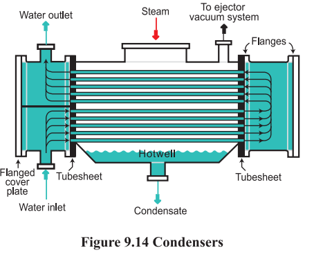
Heat Exchanger Types (by application) 

Condensers In steam applications, condensers (Figure 9.14) are associated with condensing steam turbines and with ejector systems. In steam turbine applications condensers typically operate under a vacuum. They remove significant amount of latent heat from the exhaust steam allowing it to be recovered as condensate. In steam ejector applications, condensers increase the effectiveness of the ejectors by condensing both the motive steam and condensable pilled from the process, reducing the amount of motive steam required.

Condensers can be surface type or barometric. Surface condensers are supplied with cooling water that circulates through condenser tubes providing a cool surface area that causes steam condensation. The condensate is typically collected in a condensate well, and pumped into the condensate return system. Barometric condensers rely on direct contact between the cooling water and the steam. In petroleum refining and chemical manufacturing applications, condensers are also used to condense components from gaseous mixtures. In these applications the condensers use a cooling medium to extract energy from the gases and collect the condensed components.

Distillation Towers

The petroleum refining and chemical manufacturing industries use large amount of steam to facilitate the separation of crude oil or chemical feedstocks into various components. This separation process relies on differences in the boiling points of these hydrocarbon components. Distillation towers (Figure 9.15) use a furnace to heat crude oil above 370°C. As the volatile components boil off and rise up the tower they are cooled and condensed. Steam is injected into bottom of these towers to reduce the partial pressures of the hydrocarbons, which facilitates their separation and to reduce coke formation on tray tower surfaces. 

Evaporators

Evaporators (Figure 9.16) reduce the water content of a liquid generally by heating it with steam,

in order to concentrate the product. Evaporators are used extensively in industries such as food

processing, chemical, manufacturing, steel, forest products and textiles.In most cases, evaporators are shell and tube heat exchangers with the steam on the shell side and the product being concentrated in the tubes. Evaporators can be single effect or multiple effects type. A single effect evaporator uses steam at one set of pressure and temperature conditions to boil off the vapor from product. Multiple-effect evaporators take the vapor produced from one evaporator and use it to heat the product in a lower- pressure evaporator.

Multiple Effect Evaporators

In a multiple effect arrangement, the latent heat of the vapor product off of an effect is used to heat the following effect. Effects are thus numbered beginning with the one heated by steam. It will have the highest pressure. Vapor from Effect I will be used to heat Effect II, which consequently will operate at

lower pressure. This continues through the train; pressure drops through the sequence so that the hot vapor will travel from one effect to the next.

Normally, all effects in an evaporator will be physically the same in terms of size, construction,

and heat transfer area. Unless thermal losses are significant, they will all have the same capacity as

well.

Unlike single-stage evaporators, these evaporators can be made of up to seven evaporator stages or

effects. The energy consumption for single-effect evaporators is very high and makes up most of the cost for an evaporation system. Putting together evaporators saves heat and thus requires less

energy. Adding one evaporator to the original decreases the energy consumption to nearly 50% of

the original amount. Adding another effect reduces it to nearly 33% and so on. A heat saving equation

can be used to estimate how much one will save by adding a certain amount of effects. The number

of effects in a multiple-effect evaporator is usually restricted to seven because after that, the equipment

cost starts catching up to the money saved from the energy requirement drop.

Effect of Heat Exchanger efficiency

Efficiency and productivity of many production processes inherently depend on good transfer of heat

from the heat transfer surfaces and equipment. The design technical parameters cannot often be achieved unless the heating / cooling processes are carried out efficiently.

A reduction in heat transfer that occurs almost invariably has an impact on cycle time and product

cost. To minimize adverse impact, heat exchanger performance should be monitored and maintained

at regular intervals that are determined from cost benefit criteria.

A good operation & maintenance policy therefore must be formulated right from its installation and

during subsequent years for achieving the desired process efficiency.

Pinch Analysis & Pinch Technology Application For Process & Energy Efficiency Improvements

What is Pinch ?

Consider the following simple process [Figure 9.18(a)] where feed stream to a reactor is heated before

inlet to a reactor and the product stream is to be cooled. The heating and cooling are done by use of

steam (Heat Exchanger -1) and cooling water (Heat Exchanger-2), respectively. The Temperature (T)

vs. Enthalpy (H) plot for the feed and product streams depicts the hot (Steam) and cold (CW) utility

loads when there is no vertical overlap of the hot and cold stream profiles.

An alternative, improved scheme is shown in Figure 9.18(b) where the addition of a new ‘Heat

Exchanger—3’ recovers product heat (X) to preheat the feed. The steam and cooling water requirements also get reduced by the same amount (X). The amount of heat recovered (X) depends on the ‘minimum

approach temperature’ allowed for the new exchanger. The minimum temperature approach between

the two curves on the vertical axis is ΔTmin and the point where this occurs is defined as the “pinch”.

From the T-H plot, the X amount corresponds to a ΔTmin value of 20 °C. Increasing the ΔTmin value

leads to higher utility requirements and lower area requirements.

Pinch Principle

Energy pinch identifies the minimum cost of hot utility targets, as well as the projects that allow us to

reach these targets in practice (or to get close to them).

When considering any pinch-type problem the following principles apply:

oProcesses can be defined in terms of supplies and demands (sources and sinks) of commodities

(energy, water, etc.).

o The optimal solution is achieved by appropriately matching suitable sources and

sinks.

o The defining parameter in determining the suitability of matches is quality, ie. temperature

o Inefficient transfer of resources means that the optimal solution cannot be achieved. In fact,

the amount of inefficient transfer is equal to the wasteful use of imported commodities such

as cooling water and steam.

Building the composite curves

One of the principle tools of pinch analysis involving multiple heat exchangers is the graphic

representation of composite curves (Figure 9.19), the construction of which is simple but powerful.

Composite curves are used to determine the minimum energy-consumption target for a given process.

The curves are profiles of a process’ heat availability (hot composite curve) and heat demands (coldcomposite curve). The degree to which the curves overlap is a measure of the potential for heat recovery,as illustrated in Figure 9.19.

Constructing the curves requires only a complete and consistent heat and mass balance of the process

in question. Data from the heat and mass balance are firstused to define process streams in terms of

their temperature and heating or cooling requirements

Building Composite Curves

The following are the data of heat exchangers from a process

There are two hot streams (Streams | and 2) and two cold streams (Streams 3 and 4). Note that CP is

defined as (mass flow rate) x (specific heat) and is represented by the slope of the curve in Figure

9.20 (a). For example, Stream | is cooled from 200°C to 100°C, releasing 2000 kW of heat, and so

has a CP of 20 kW/°C,

Figure 9.20 (a) shows the hot streams plotted separately on a temperature-duty diagram. The hot

composite curve in Figure 9.20 (b) is constructed by simply adding the enthalpy changes of the

individual streams within each temperature interval. In the temperature interval 200°C to 150°C, only

Stream | is present. Therefore, the CP of the composite curve equals the CP of Stream 1, i.e., 20. In

the temperature interval 150°C to 100°C, both Streams 1 and 2 are present. Here, the CP of the hot

composite is the sum of the CPs of the two streams, i.e., 20+40=60. In the temperature interval 100°C

to 60°C, only Stream 2 is present, so the CP of the composite is 40.

Construction of the cold composite curve is done similarly to that of the hot composite curve, but

combines the temperature enthalpy curves of the cold streams (see Figures 9.21 (c) and (d)).

Determining the energy targets

To determine the minimum energy target for the process, the cold composite curve is progressively

moved toward the hot composite curve, as shown in Figure 9.22 (a). Note that the enthalpy axis measures relative quantities, which means that we are representing the enthalpy change of process

streams. Moving a composite curve horizontally does not, in any way, change the stream data. The

closest approach of the curves is defined by the minimum allowable temperature difference, ΔTmin

(Figure 9.22 (a)). This value determines the minimum temperature difference that will be accepted in

a heat exchanger. A value of 10°C has been used in this example.

The overlap between the composite curves shows the maximum possible process-heat recovery

(as shown in Figure 9.22 (b)), indicating that the remaining heating and cooling needs are the minimum

hot utility requirement (QHmin) and the minimum cold utility requirement (QCmin) of the process

for the chosen ATmin. In this example, the minimum hot utility (QHmin) is 900 kW and the minimum

cold utility (QCmin) is 750 kW.

Using pinch analysis, targets can be set for minimum energy consumption prior to any heat exchanger

network design. This enables quick identification of the scope for energy savings, at an early stage of

the analysis. This single benefit is likely to be the biggest strength of the approach.

Benefits and Applications of Pinch Technology

One of the main advantages of Pinch Technology over conventional design methods is the ability to

set energy and capital cost targets for an individual process or for an entire production site ahead of

design. Therefore, in advance of identifying any projects, the scope for energy savings and investment

requirements can be determined.

General Process Improvements

In addition to energy conservation studies, Pinch Technology enables process engineers to achieve the

following general process improvements:

Update or Modify Process Flow Diagrams (PFDs): Pinch quantifies the savings available by changing the process itself. It shows where process changes reduce the overall energy target, not just local energy consumption.

Conduct Process Simulation Studies: Pinch replaces the old energy studies with information that

can be easily updated using simulation. Such simulation studies can help avoid unnecessary capital

costs by identifying energy savings with a smaller investment before the projects are implemented.

Set Practical Targets: By taking into account practical constraints (difficult fluids, layout, safety, etc.),

theoretical targets are modified so that they can be realistically achieved. Comparing practical with

theoretical targets quantifies opportunities “lost” by constraints - a vital insight for long-term

development.

Debottlenecking: Pinch Analysis, when specifically applied to debottlenecking studies, can lead to

the following benefits compared to a conventional revamp:

1.Reduction in capital costs

2.Decrease in specific energy demand giving a more competitive production facility

For example, debottlenecking of distillation columns by Column Targeting can be used to identify

alternate, cost effective options to column re-traying or installation of a new column.

Determine Opportunities for Combined Heat and Power (CHP) Generation: A well-designed

CHP system significantly reduces power costs. Pinch shows the best type of CHP system that matches

the inherent thermodynamic opportunities on the site. Unnecessary investments and operating costs

can be avoided by sizing plants to supply energy that takes heat recovery into consideration. Heat

recovery should be optimized by Pinch Analysis before specifying CHP systems.

Decide what to do with low-grade waste heat: Pinch shows, which waste heat streams, can be

recovered and lends insight into the most effective means of recovery.

Solved Example:

A counter-flow double pipe heat exchanger using hot process liquid is used to heat water, which flows

at 10.5m°?/hr. The process liquid enters the heat exchanger at 180°C and leaves at 130°C. The inlet and

exit temperature of water are 30°C and 90°C respectively. Specific heat of water is 4.18 kJ/kg°C.

a) Calculate the heat transfer area, if overall heat transfer coefficient is 814 W/m7°C.

b) What would be the percentage increase in are, if the fluid flows were parallel?

--------------------------------

Chapter 1